Delving Deeper Into LlamaIndex: An Inside Look

Unmasking the mechanics of GitHub repository indexing

(Image generated by Midjourney)

In my previous piece about LlamaIndex, we walked through a simple use case of indexing a GitHub repository to be able to ask questions about it. I thought it would be interesting to delve deeper and try to understand what it does in a bit more detail. I believe this is useful for two reasons. Firstly, LlamaIndex is highly customizable and extensible and by fully understanding how it works in one particular application, we’ll be much better positioned to apply it to another. The second reason is that, if you played around with the demo from the previous article, you might have come against some limitations. We’ll come back to them at the end, but as we learn more about LlamaIndex, we’ll hopefully see why those happen and what we can do to avoid them.

Firstly, let's quickly recap what our llamaindex-demo does, or rather, what LlamaIndex does for us:

LlamaIndex workflow

In our example, we broke the workflow in two — ingestion (marked in green) and querying (marked in blue). I’d like to start at the end by diving into what happens when we make a query. Then we can work our way through the ingestion steps to figure out how we get there.

Query workflow

To test out how querying works I enabled debug-level logging in query.py:

import logging
logging.basicConfig(stream=sys.stdout, level=logging.DEBUG)
logging.getLogger().addHandler(logging.StreamHandler(stream=sys.stdout))

Now when running the script, it prints a lot of information which helps us understand exactly what it’s doing. I’ve added the entire log to the GitHub repo here but in summary, we can see it does the following:

1. Load the index we previously created by running index.py
2. Invoke the OpenAI API to fetch the embedding for the question posed in the program “What does load_index_from_storage do and how does it work?”. It uses the text-embedding-ada-002 model and returns an embedding vector.
3. With the embedding, it looks up the two nodes with most similar embeddings. These happen to be in llama_index/storage/index_store/types.py and llama_index/indices/loading.py.
4. Invoke the OpenAI API again but this time the completions endpoint with a prompt using content of the nodes it found. It uses the text-davinci-003 model with a temperature (how wild the answers can be) of 0.0 (not wild at all) and max_tokens (how long the response can be) of 256.
5. The last call returns the final answer which is displayed to the user.

There are a couple of interesting details. Firstly, how did the lookup in the vector store happen to hit some nodes relevant to our question? I’ll come to that later. The second question is what was in the prompt which got fed into text-davinci-003 (basically, GPT-3) which led to the (correct) answer? We can see that in the debug output too:

Context information is below. 
---------------------
file_path: llama_index/storage/index_store/types.py
file_name: types.py

from abc import ABC, abstractmethod
from typing import List, Optional

from llama_index.data_structs.data_structs import IndexStruct
...

file_path: llama_index/indices/loading.py
file_name: loading.py
...
    if index_ids is None:
        logger.info("Loading all indices.")
        index_structs = storage_context.index_store.index_structs()
    else:
        logger.info(f"Loading indices with ids: {index_ids}")
        index_structs = []
        for index_id in index_ids:
            index_struct = storage_context.index_store.get_index_struct(index_id)
            if index_struct is None:
                raise ValueError(f"Failed to load index with ID {index_id}")
---------------------
Given the context information and not prior knowledge, answer the question: What does load_index_from_storage do and how does it work?

I’ve truncated it but you can find the full prompt here. We can take the prompt and paste it into the OpenAI playground. For fun, I thought I’d see what happened if I dialed up the temperature:

Temperature at 2: Don’t go there!

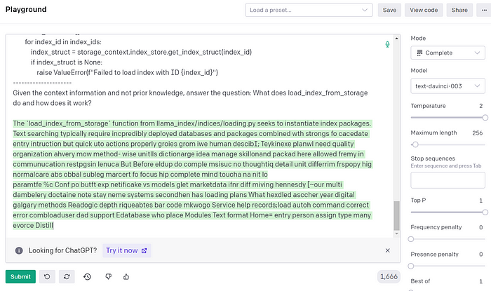
For the kinds of applications we’re building here, we just want it to summarize the hard facts so setting the temperature to 0 avoids any hallucinations and forces the model to rely entirely on the context. Here’s what the whole workflow looks like:

Query workflow

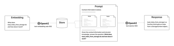
The Store here is the same one as in the first diagram containing the nodes we ingested — we’ll cover how it’s populated later. See how, there are two separate calls to two different OpenAI models — the first to fetch the embedding for the question, the second to GPT 3 to ask it to complete our question given the context.

You might be interested to know how much it cost (I was because I just paid for it). From the debug output, I can see it used 16 tokens to fetch the embedding which, at 0.0004/1k tokens would be $0.0000064 — I’m not sweating yet. For the completion though, 1551 tokens, at $0.02/1k tokens come in at $0.03 which is not free but certainly cheaper than loading than trying to load the entire codebase into GPT-4 (32k) to ask the query. Assuming the codebase would fit into 32k tokens (it wouldn’t), the query would have cost $1.92.

Right, I think that covers the query workflow. Now to address where the nodes come from, let’s rewind to the beginning and examine step-by-step how ingestion works.

Ingestion

1. Load

In llamaindex-demo, we did the following to “load” the data from a GitHub repo:

loader = GithubRepositoryReader(..., repo="llama_index", ...)
docs = loader.load_data(branch="main")

Besides the GitHubRepositoryReader we used here, there are a tonne of different readers to choose from. Each one connects to a different source (Slack, Notion, Wikipedia, a database, etc.) and provides a load_data method which reads the source documents and returns a List[Document]. What’s a Document? Here’s the signature:

@dataclass
class Document:
    text: str      # The content of the document 
    doc_id: str    # A unique identifier for the document
    doc_hash: str  # A hash of the content
    extra_info: Dict[str, Any] # Extra metadata about the document

What gets stored in extra_info is up to the loader. In the case of GithubRepositoryReader it stores the file path and filename. So to illustrate a single example from the llama_index repository:

A Document representing a Python source file

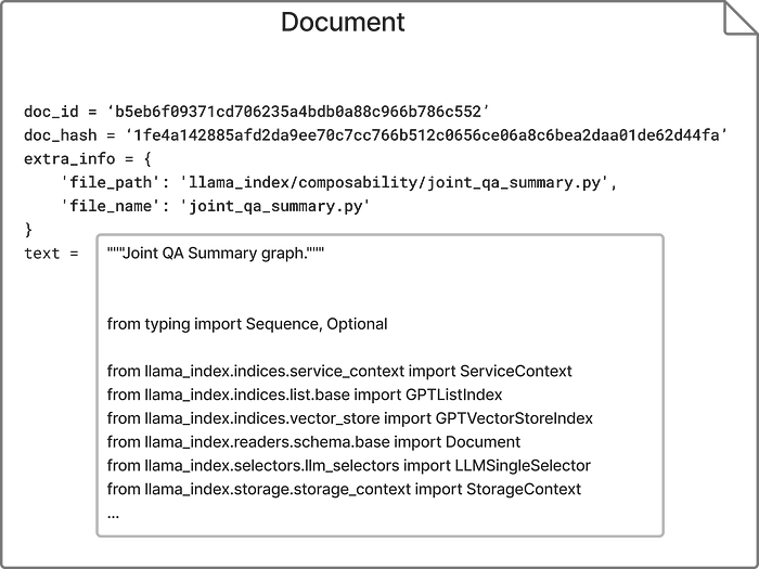
Thus, after completing step 1. of our ingestion script, we now have a list of Document objects each containing the content of a source file in the llama_index repository along with an ID if we want to persist it, a hash to check if a previously persisted version differs from a newly read one, and the file’s path and name.

Next, let's look at what it means to parse all those documents.

2. Parse

In our demo, we did:

parser = SimpleNodeParser()
nodes = parser.get_nodes_from_documents(docs)

LlamaIndex only comes with SimpleNodeParserbut we can make our own if we prefer. A parser has to implement aget_nodes_from_documents method which takes a Sequence[Document] and returns a List[Node]. So what’s a Node?

@dataclass
class Node(Document):
    node_info: Dict[str, Any]
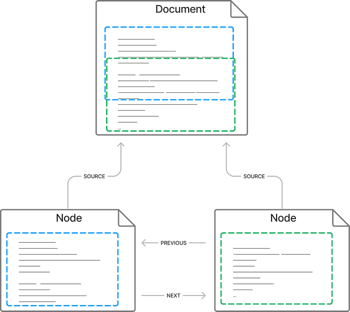
    relationships: Dict[DocumentRelationship, Any]

A node is a document but with some extra information. It says what relationships it has to other nodes or documents — PREVIOUS, NEXTor SOURCE(nodes can also have parent-child relationships but we’re not using those here) and information about where the node comes from such as the position. The real point of a node though is that it’s a small enough chunk for which to create an embedding (Ada has a cap of 2,049 tokens) and then recall and use in the completion.

SimpleNodeParser is basically a chunker of entire documents into smaller (default 4000 characters) nodes but with a couple of features that make the querying more useful. For example, it will split at whitespace otherwise words like “outside” might get split into “out” and “side” and end up treated as different tokens with a different meaning. Also, it will create overlapping chunks — that is, the second node will include the end of the first, and the beginning of the third etc. The purpose of this overlap is that if a fact needs to be recalled from the boundary of a node, it should also exist in a neighbour node. Both nodes should be retrieved later in a query about that fact and, between them, there should be enough context to support the fact.

Hopefully, this will make it clearer:

Relationships between Nodes and Document

Now we have a bunch of Nodes, we can index them.

3. Index

In llamaindex-demo, we did:

index = GPTVectorStoreIndex(nodes)

This iterates over every node and invokes OpenAI’s text-embedding-ada-002 model to fetch an embedding vector for each node. You may recall this is the same model which gets used to fetch the embedding for the query and it has to be. You can’t compare embeddings from one model with embeddings from another.

Because of all those calls to OpenAI to fetch the embeddings, this is the most expensive part of the process. To index the llama-index repo, it currently consumes 503,314 tokens which, at $0.0004/1k tokens add up to $0.20. The good news is because we persist the index in the next step, we only need to run this once.

4. Persist

In our ingest.py demo, we did the following to persist the index:

index.storage_context.persist(persist_dir="index")

This uses the default implementation which persists all the nodes, some indices, and embeddings in JSON files so that the whole lot can be read back next time. We touched on this briefly in the previous article and I don’t think there’s much more to dig into. However, while the default store works well for our relatively small demo, for large datasets, it may be impractical to read the whole store back into memory again. LlamaIndex has support for lots of 3rd party vector databases such as FAISS and Pinecone. If you’re not familiar with this new breed of databases, I’ll explain why they’re useful in the next section.

Querying the store

We’ve come full circle from querying, back to ingestion, and now to querying again because, while I explained the query workflow, I didn’t explain how relevant nodes for a query are actually found.

We’ve learned that during ingestion, OpenAI is queried to give each node an embedding. Similarly, when we run a query, we again query OpenAI for an embedding. The magic of embeddings is that given two quite different pieces of text about the same thing e.g.:

1. A question about load_index_from_storage
2. The code definition of load_index_from_storage

The embeddings should be more similar than any two pieces of text about different things (if you didn’t read this article about embeddings last time, I encourage you to do so now). So what we need to do is, given the embedding of our question, find the “nearest neighbours” in the multi-dimensional embedding space containing all our nodes. We pick the closest two (we want at least two so we capture the complete context if the fact we’re looking for is at the border of two nodes) and they become the context for our LLM query.

What makes vector databases like Pinecone hot at the moment is that they’re optimized specifically for this job of storing nodes with embeddings (i.e. vectors) as indices and looking up the nearest neighbours.

Conclusion

Hopefully, this has helped you learn how LlamaIndex works — writing this certainly helped me understand at least. What I also found interesting along this journey were the opportunities to improve the solution such as:

1. SimpleNodeParser is designed for chunking natural language. In the case of code, however, there are natural chunk boundaries in the form of methods or functions. For queries about a particular method, there’s little point providing bits of other methods in the context, nor splitting the method up. A code-specific could do a much better job but it would also be more complicated because it would have to understand the syntax of the programming language it was parsing.
2. The knowledge-retrieval mechanism of LlamaIndex is designed to retrieve a couple of items of knowledge for the query prompt but what if the query concerns the overall architecture of the codebase? I can think of different approaches to this problem e.g. feeding all (or at least very large chunks) of the codebase to a prompt to generate summaries.

I’ll be exploring these ideas in future articles so stay tuned!

In the meantime, you may want to check out the part2 branch I made to the repository from the previous article.