Working With Payments Data in Python and SQL
Introducing the bins and buckets problem

One of the industry's most common data analyst and data engineering problems is working with accounting data. This is for a simple reason: every business with customers needs to invoice them for services (charges) and then collect them on those invoices (payments).
Every. Business.
Since collecting on payments for services rendered is the lifeblood of a business, understanding how those collections are going, analyzing who is paying (or not paying), and reporting this information to senior management is a very common data task that a data analyst and/or data engineer will be responsible for.
Some of these tasks may be outsourced to an accounting product like QuickBooks by Inuit or an industry-specific tool like Yardi for the real estate industry. While these products may have some analytic functionality out of the box, any custom analysis will require pulling the raw data, cleaning it, and pipelining it to a report deliverable (dashboard, slide deck, etc.).
As an example of where this can be critical: it’s late 2020 in the United States, and your apartment leasing company has just received word that there will be a moratorium on evictions. Senior management wants a detailed check on how this has affected rent collection by market, by age, by everything. Base functionality on Yardi is not going to cut it.
You pull up the API reference for your company’s accounting software and see that for each customer, you can access a transaction-level record of payments with the payment date and a record of each invoice instance with the bill date. Now, just to put them together. Easy, right?
Until you realize that customer 27139 doesn’t pay on time and when the customer does pay, it is in small amounts sometimes and big amounts other times, such that sometimes 27139 underpays for the month but sometimes overpays for the month. Which month?! All you have is the payment date and the amount, not the specific invoice to which it is being credited. You explore and realize this problem is not unique to 27139; it’s tons of customers. What do you do?
In this tutorial, I am going to do three things:
- Demonstrate how to solve this fundamental challenge with payment data using Python and SQL.
- Contrast the approach between Python and SQL to provide a concrete example of the differences in programming between Python and SQL. The fundamental logic needed to program in these two languages goes beyond syntax.
- Use this as an example of the type of work you might find in the industry as a data analyst. This will complement simpler problems aspiring data analysts typically find in course materials.
Accompanying GitHub Notebook Available
The Fundamental Challenge
The common issue when working with charge and payment data is that the charges and payments will be recorded at a transaction level as a stream of records with an amount, a date, and an account number. At some point, however, individual transaction data needs to be matched between payments and charges so late fees can be assessed if appropriate, payment behavior among customers can be aggregated for reporting, cash flow analysis, and similar tasks. The core problem is allocating a payment transaction (in part or in full) to the appropriate charged invoice based on the bill date.
Here is an example of what this data may look like in the rawest form.
Charge/invoice data

Payment data
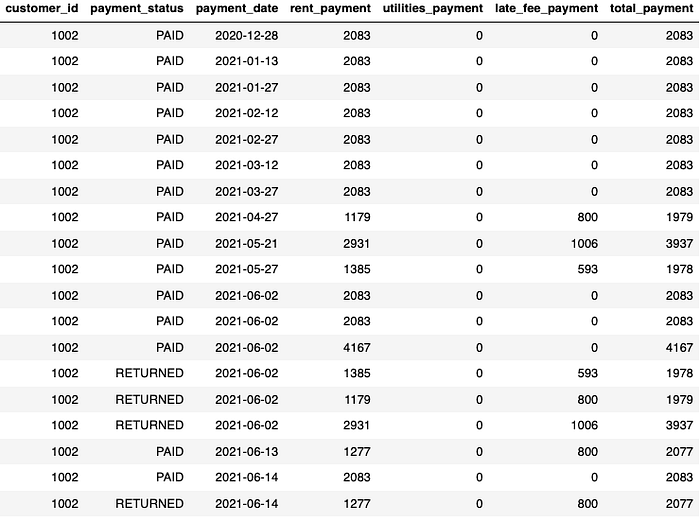
As a human, you can spend some time going through this account’s information, piece together what happened, and sort it out, but that approach does not scale, and we need to use code to make it possible to do this match for millions or billions of records. Here is what the final allocation should look like if you want to try it by hand and check your work.
Allocated payments

To build an intuition for the approach to this problem, let’s abstract it to a simpler setting that operates similarly and solve the problem in that setting first. The problem is one of First In, First Out allocation. In other words, we have a stream of payments that come into our records, and those payments must be allocated in the order they arrive with the charges ordered by their bill dates.
An equivalent problem is having an ordered sequence of buckets of water and an ordered sequence of empty bins. How can we algorithmically transfer the water from the buckets to the bins while preserving the order of both?
Introducing the Bins and Buckets Problem
In the Bins and Buckets problem, we have two core elements:
- Some buckets with varying volumes are filled with water and ordered
- Some empty bins, possibly of varying capacities, are ordered.
We wish to transfer the water from the buckets in the order they are labelled to the bins in the order they are labelled. The ultimate goal is to make it so each bucket is sequentially poured into the bin with the lowest number that has not been filled yet and keep doing this until all the buckets are emptied or all the bins are filled.
Consider we have the following buckets with accompanying volumes of water:
- Bucket 0: 2 Liters
- Bucket 1: 3 Liters
- Bucket 2: 5 Liters
- Bucket 3: 2 Liters
- Bucket 4: 1 Liter
- Bucket 5: 4 Liters
- Bucket 6: 5 Liters
We also have the following Bins with accompanying capacity:
- Bin 0: 5 Liters
- Bin 1: 6 Liters
- Bin 2: 8 Liters
- Bin 3: 4 Liters
- Bin 4: 6 Liters
We have a total of 22 Liters of water and 30 Liters of capacity, so clearly, we end up in a situation where we exhaust the amount of water available before we exhaust the available capacity. When we do the allocation, we get the following easily verified result.
Note: bucket_ind represents the bucket number, bin_ind represents the bin number, and the amount column refers to the allocated amount from the bucket to the corresponding bin.

This is equivalent to the charges and payments problem, where the buckets represent the payments, and the bins represent the charges. We order payments and charges by their respective dates, then allocate them to charges in order until each charge is “full” before moving on to the next charge. By solving the Bins and Buckets problem, we are simultaneously solving the payment allocation problem.
How do we do this algorithmically/programmatically in Python?
If you solved the example above by hand, you’ve probably already stumbled on the algorithm.
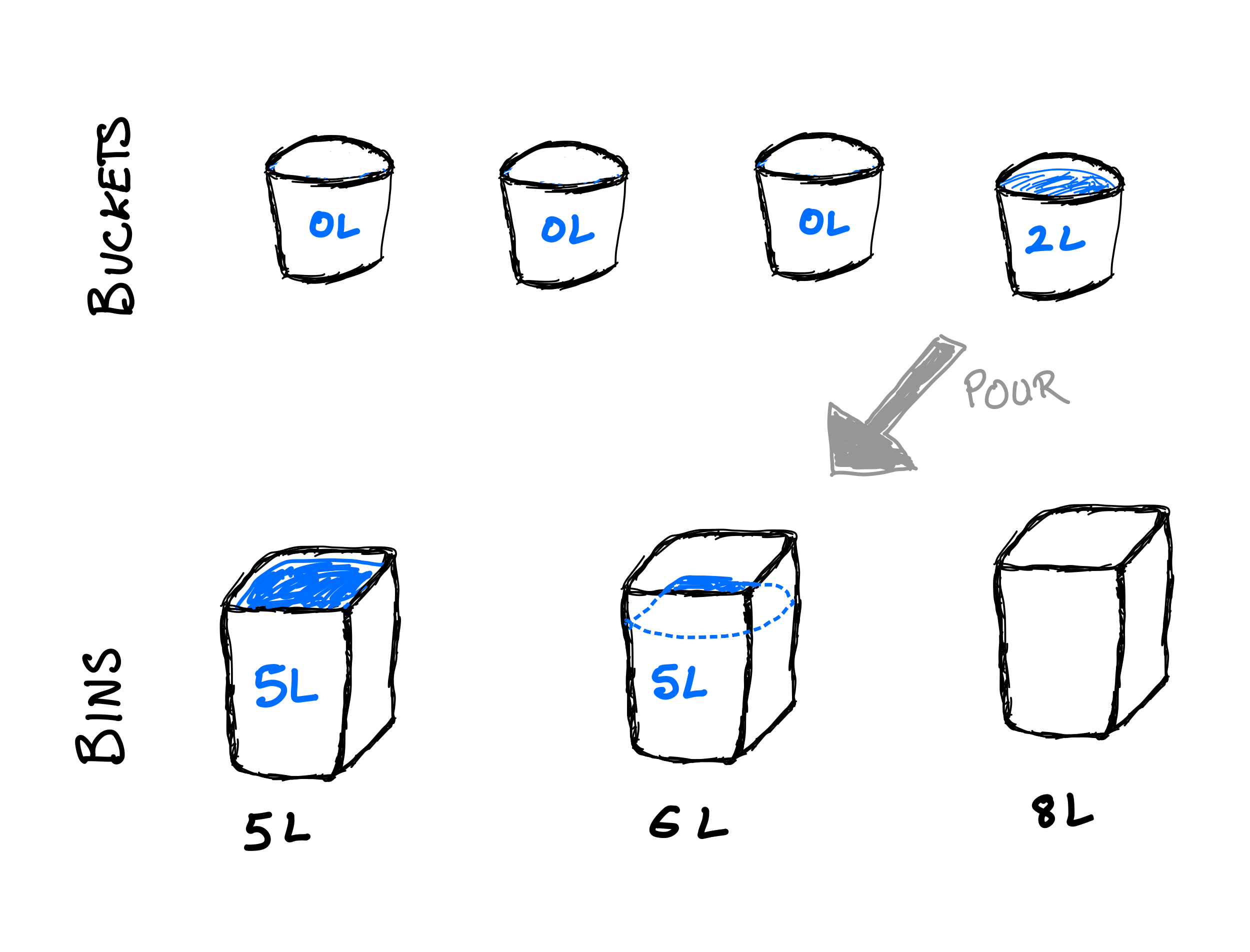
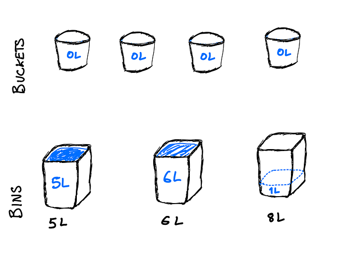
We start with the first bucket and the first bin. We pour the water from the bucket into the bin until either the bucket is empty or the bin is full, whichever happens first. If the bucket empties first, we select the next and repeat. If the bin fills first, we stop pouring into the bin and start pouring the remaining water into the next bin and repeat. Along the way, we record which buckets are matched to which bins and how much water is allocated.
The algorithm can be shown visually using the first few bins and buckets from the example above:



We can then put this into code in Python.
bucket_allocation = list() # tuples (bucket_index, bin_index, amount of allocation)

exit_flag = False
# Set up iterator for buckets
current_bucket_idx = 0
# Set up dynamic tracker for bucket contents
buckets_tracker = buckets.copy()

# Iterate through each bin as main unit
for i, bin_i in enumerate(bins):

    if exit_flag:
        break

    # While the current bin still has capacity for more water
    while bin_i > 0:

        # If the current bucket under review has less (or equal) water than the current capacity in the bin
        if buckets_tracker[current_bucket_idx] <= bin_i:
            # 1. Update the allocation so that the bucket empties all its contents into the bin
            bucket_allocation.append((current_bucket_idx, i, buckets_tracker[current_bucket_idx]))
            # 2. Update the capacity of the bin to account for the water added
            bin_i = bin_i - buckets_tracker[current_bucket_idx]
            # 3. Update the bucket tracker to note there is no more water in the bucket
            buckets_tracker[current_bucket_idx] = 0
            # 4. Iterate the bucket tracker to move onto the next bucket
            current_bucket_idx += 1

            # Exit if we run out of buckets
            if current_bucket_idx >= len(buckets_tracker):
                exit_flag = True
                break

        else:
        # If the current bucket has more water than the capacity of the current bin
            # 1. Update the allocation so that the bucket empties only to the current remaining capacity of the bin
            bucket_allocation.append((current_bucket_idx, i, bin_i))
            # 2. Update the bucket tracker to record the removed water added to the current bin
            buckets_tracker[current_bucket_idx] = buckets_tracker[current_bucket_idx] - bin_i
            # 3. Update the bin capacity to be zero so we can move onto the next bin
            bin_i = 0
Running this code with the bins and buckets from the above example will return the allocations as shown. You can play around with the inputs in the Notebook available on GitHub.
How do we do this algorithmically/programmatically in SQL?
What do you mean, “how”? Didn’t we already solve this above? Let’s just copy the logic to the SQL syntax. Now, uh, where is that for loop in SQL…?
This is the foundational difference between working in Python and in a SQL (database) environment: Databases operate exclusively in “tables,” whereas a general programming environment like Python is very flexible in its data structures and algorithmic logic. In the algorithm we illustrated above, we map how we would do this in the real world onto a programmatic execution of that logic. In the real world, we are not constrained to think in terms of tables and rows but in a database context we are.
To understand how to do this in SQL, we must carefully understand what information we are encoding in the Python implementation (and our IRL approach). We are inputting data about the size of the respective bins and buckets, and we are outputting the allocation of that data. However, what we are *encoding* in the implementation through the data structure is the state of the bins and buckets with each action.
The for loop and the dynamically updating list structures allow us to iterate through each bin and bucket one by one, take an action, and update the system state sequentially for each action. In a table environment, we cannot implicitly store these sequential actions in a dynamically updating data structure. Tables require simultaneous updating as SQL functions apply across all rows simultaneously (or a sort of middle ground between simultaneously and sequentially in the case of window functions).
To tackle this, we need to think of another way to capture the encoded information but without sequentially updating the system's state.
What system information are we encoding with the Python data structures? Essentially, we are storing information about the cumulative amount of water poured from the buckets and the cumulative amount of capacity used from the bins. Here is what is happening in the toy example above with some additional perspective.


Fortunately for us, tracking a cumulative sum is very easy to do in SQL. We can do this with the following SQL code for the buckets. We use SUM as a window function and COALESCE to fill in the 0 for the first prev_cumulative_water, which gets returned as a NULL by the SUM function here. (It will become clear later why we also include the prev_cumulative columns if it is not already.)
SELECT
    bucket_ind,
    water,
    SUM(water) OVER (
        ORDER BY bucket_ind ASC ROWS BETWEEN UNBOUNDED PRECEDING AND CURRENT ROW
    ) AS water_cum,
    COALESCE(SUM(water) OVER (
        ORDER BY bucket_ind ASC ROWS BETWEEN UNBOUNDED PRECEDING AND 1 PRECEDING
    ),0) AS prev_water_cum
FROM buckets
The code for the bins is almost identical, so I won’t reproduce it here, but it is available in the Notebook. Here is what the code output for both the bins and buckets tables looks like:

The next challenge we have is how to match up the buckets to the correct bins. In the Python case, we poured a bucket into a bin until it was full and then proceeded with the next bucket. But, as discussed above, we do not have the list data structure to manage this matching implicitly; we need to do it explicitly.
The challenge of comparing cumulative water and cumulative capacity requires us to make a join between the two tables without knowing how to correctly join the tables until we make the join.
To manage this, we join every bucket to every bin and check if that bin and bucket should be matched using cumulative data afterward. SQL makes this very easy to do with its CROSS JOIN function. It does exactly this.
WITH buckets_data AS (
    SELECT
        bucket_ind,
        water,
        SUM(water) OVER (
            ORDER BY bucket_ind ASC ROWS BETWEEN UNBOUNDED PRECEDING AND CURRENT ROW
        ) AS water_cum,
        COALESCE(SUM(water) OVER (
            ORDER BY bucket_ind ASC ROWS BETWEEN UNBOUNDED PRECEDING AND 1 PRECEDING
        ),0) AS prev_water_cum
    FROM buckets
), bins_data AS (
    SELECT
        bin_ind,
        capacity,
        SUM(capacity) OVER (
            ORDER BY bin_ind ASC ROWS BETWEEN UNBOUNDED PRECEDING and CURRENT ROW
        ) AS capacity_cum,
        COALESCE(SUM(capacity) OVER (
            ORDER BY bin_ind ASC ROWS BETWEEN UNBOUNDED PRECEDING and 1 PRECEDING
        ), 0) AS prev_capacity_cum
    FROM
        bins
)
SELECT
    *
FROM
    buckets_data
    CROSS JOIN bins_data
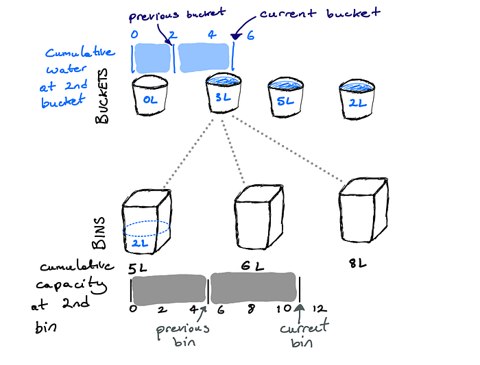
We now need to filter the table to find the appropriate bin-bucket rows that correctly match buckets to bins. To do this, we need to use the cumulative data the list structure was implicitly encoding for us in the Python approach. To illustrate how we do this, let’s consider the system’s state after we pour the first bucket into the first bin and then focus on the second bucket.

We know that in the final allocation, the second bucket (Bucket 1) must be matched to the first bin (Bin 0), but at this point, we must consider it potentially matched to any of the bins. The first three of these are shown in our illustration.
We need to figure out how to positively select the first bin for the bucket while also negatively selecting the second and third bins (i.e. do not match to the second and third bins). We use the cumulative water (or capacity) information to do this. In particular, we make use of the cumulative water (or capacity) information up to and including the bucket (or bin), and the cumulative water (or capacity) information up to but not including the bucket (or bin). This will help us determine the “previous cumulative” point.
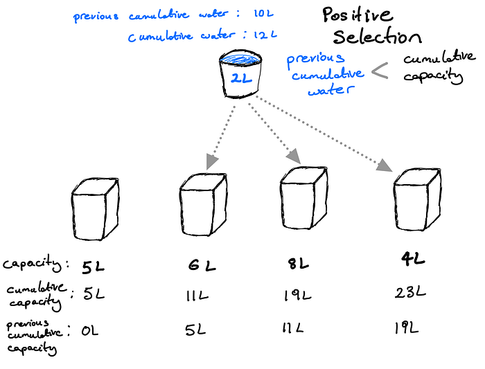
We start by illustrating the criteria for positive selection.
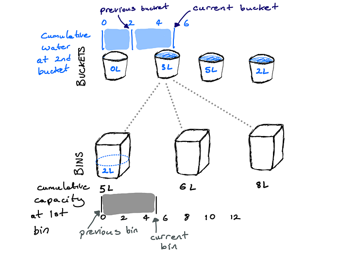
For the second bucket, the cumulative water (up to and including the bucket) is 5L, while the previous cumulative water (not including the current bucket) is 2L. For the first bin (Bin 0), the cumulative capacity (up to and including the bin) is 5L, while the previous cumulative capacity (not including the current bin) is 0L since there is not a previous bin.
If the cumulative capacity of this bin (5L) is greater than the amount of previous cumulative water added (2L), then this bin must have the capacity for more water so we can select it to receive more water. This reasoning would also select the second and third bins since the cumulative capacity of these bins is also greater than the previous cumulative water added for Bucket 1. We need to negatively select for these bins.
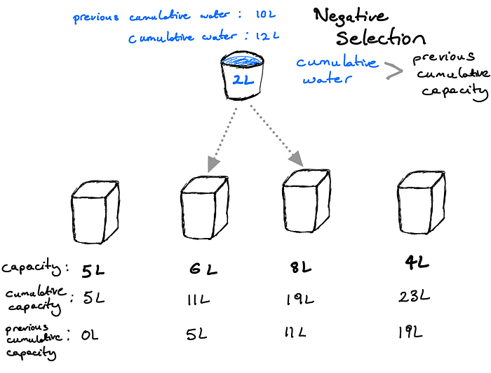
We do this by examining the bucket's cumulative water compared to the previous cumulative capacity of these bins. For instance, consider Bin 1 (the second bin). The cumulative capacity at Bin 1 is 11L, and the previous cumulative capacity is 5L.
For Bucket 1 to have enough water to fill into Bin 1, Bucket 1 must have cumulative water greater than the previous cumulative capacity at Bin 1, i.e., cumulative water greater than 5L. This is clear by noting that the cumulative water of Bucket 1 is 5L and the previous cumulative capacity at Bin 1 is also 5L, so it cannot be the case that after pouring Bucket 1 into the bins previous to Bin 1, we would have any water left over to pour into Bin 1. The same reasoning would eliminate Bin 2 and all later bins, so we have found a way to negatively select these bins.
Therefore, to positively select bins that are available to receive water from a given bucket, we filter the bin-bucket rows by selecting rows where the previous cumulative water for the bucket is less than the cumulative capacity of the bin. To negatively select buckets that will not have any water available to be poured into a given bin, we filter the bin-bucket rows by selecting rows where the cumulative water is greater than the previous cumulative capacity for the bin.
These two criteria provide us with the correct bin-bucket matches. For additional clarity, let’s examine how these two rules operate on Bucket 3.
The SQL code that does this is shown below, and the corresponding output is presented. You can note how it matches the bin-bucket rows from the Python algorithm.
WITH buckets_data AS (
    SELECT
        bucket_ind,
        water,
        SUM(water) OVER (
            ORDER BY bucket_ind ASC ROWS BETWEEN UNBOUNDED PRECEDING AND CURRENT ROW
        ) AS water_cum,
        COALESCE(SUM(water) OVER (
            ORDER BY bucket_ind ASC ROWS BETWEEN UNBOUNDED PRECEDING AND 1 PRECEDING
        ),0) AS prev_water_cum
    FROM buckets
), bins_data AS (
    SELECT
        bin_ind,
        capacity,
        SUM(capacity) OVER (
            ORDER BY bin_ind ASC ROWS BETWEEN UNBOUNDED PRECEDING and CURRENT ROW
        ) AS capacity_cum,
        COALESCE(SUM(capacity) OVER (
            ORDER BY bin_ind ASC ROWS BETWEEN UNBOUNDED PRECEDING and 1 PRECEDING
        ), 0) AS prev_capacity_cum
    FROM
        bins
)
SELECT
    bucket_ind,
    bin_ind,
    water,
    capacity,
    water_cum,
    capacity_cum,
    prev_water_cum,
    prev_capacity_cum
FROM
    buckets_data
    CROSS JOIN bins_data
WHERE
    prev_water_cum < capacity_cum
    AND water_cum > prev_capacity_cum
Now that we have identified the correct bin-bucket rows, we need to calculate the specific water allocation from each bucket to the corresponding bin(s). This algorithm follows the corresponding Python step fairly closely; we need to identify how much water is available for the bin and if the water exceeds the capacity available in the bin. We do this as follows:
- Identify the “current balance” between water and capacity. The current balance differs between the bucket's previous cumulative water and the bin's cumulative capacity. This tells us whether there is any excess water or capacity up to this point in the matched bins and buckets.
- Make an update to either capacity or water based on the current balance:
- If the current balance is greater than or equal to 0, we have more water. The bin must already hold this excess water, so we have to update the available capacity in the bin to account for it. The updated capacity will differ between the bin’s capacity and the current balance.
- If the current balance is less than 0, we have more capacity. This excess cumulative capacity implies that some water from the bucket must be allocated to this excess capacity. We have to update the available water in the bucket for allocation to the bin associated with the row. The updated water will be the difference between the bucket’s water and the absolute value of the current balance.
- Allocate the water from the bucket to the bin. We compare the relevant value for capacity (either total capacity or updated capacity) with the relevant value for water (either the total water or updated water). If the capacity is greater than or equal to the water, then the water value is allocated to the bin. If not, only the amount of water equal to the capacity is allocated.
The SQL code implements that logic combined with all the previous data preparation steps and the corresponding output.
WITH buckets_data AS (
    SELECT
        bucket_ind,
        water,
        SUM(water) OVER (
            ORDER BY bucket_ind ASC ROWS BETWEEN UNBOUNDED PRECEDING AND CURRENT ROW
        ) AS water_cum,
        COALESCE(SUM(water) OVER (
            ORDER BY bucket_ind ASC ROWS BETWEEN UNBOUNDED PRECEDING AND 1 PRECEDING
        ),0) AS prev_water_cum
    FROM buckets
), bins_data AS (
    SELECT
        bin_ind,
        capacity,
        SUM(capacity) OVER (
            ORDER BY bin_ind ASC ROWS BETWEEN UNBOUNDED PRECEDING and CURRENT ROW
        ) AS capacity_cum,
        COALESCE(SUM(capacity) OVER (
            ORDER BY bin_ind ASC ROWS BETWEEN UNBOUNDED PRECEDING and 1 PRECEDING
        ), 0) AS prev_capacity_cum
    FROM
        bins
)
SELECT
    *,
    CASE
        WHEN current_balance >= 0 THEN IIF(
            updated_capacity >= water,
            water,
            updated_capacity
        )
        WHEN current_balance < 0 THEN IIF(
            capacity >= updated_water,
            updated_water,
            capacity
        )
        ELSE 0
    END AS water_allocation
FROM (
    SELECT
        bucket_ind,
        bin_ind,
        water,
        capacity,
        water_cum,
        capacity_cum,
        prev_water_cum,
        prev_capacity_cum,
        prev_water_cum - prev_capacity_cum AS current_balance,
        IIF(
            prev_water_cum - prev_capacity_cum >= 0,
            capacity - (prev_water_cum - prev_capacity_cum),
            NULL
        ) AS updated_capacity,
        IIF(
            prev_water_cum - prev_capacity_cum < 0,
            water + (prev_water_cum - prev_capacity_cum),
            NULL
        ) AS updated_water
    FROM
        buckets_data
        CROSS JOIN bins_data
    WHERE
        prev_water_cum < capacity_cum
        AND water_cum > prev_capacity_cum
) data
You can verify that it is the same as the Python results.
Now that we have explored the solutions to the Bins and Buckets problem in Python and SQL, we can briefly revisit the original problem. How do we allocate payments to charges?
The code above can be easily adapted to solve this problem with just a bit more functionality to manage:
- The
RETURNEDpayments need to be removed from the payments record. - The Bins and Buckets solution need to be adapted to work across multiple accounts; it is currently designed to work on records for a single account.
The second bullet is handled in code in the accompanying Notebook for SQL and Python. The first bullet is handled in Python in the Notebook. It can also be done in SQL but varies depending on how returned payment records are coded in the data, so I am only writing code to manage it to show how to allocate the payments to the charges.
Please visit the Notebook on GitHub if you want to see the code adapted to the payment and charge data. In the next image, I will remind you of the inputs and outputs for the task:
Charge data

(Cleaned) payments data
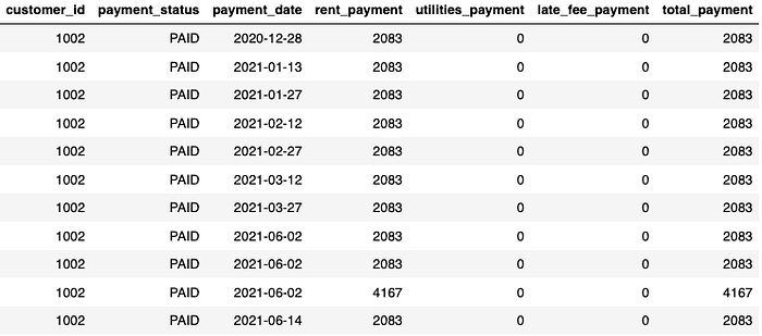
Allocated payment records

Comparison of Python and SQL
In an article for Data Camp, the author discusses high-level ideas about the two languages and asks, “SQL vs Python: Which Should You Learn?” He answers the question in part as follows:
“SQL is certainly an easier language to learn than Python. It has a very basic syntax that has the sole purpose of communicating with relational databases. Since a great amount of data is stored in relational databases, retrieving data using SQL queries is often the first step in any data analysis project. Learning SQL is also a great choice because it will help you interiorize basic concepts of programming in a user-friendly way, paving your way to move to more complex programming languages.”
In a head-to-head comparison of the advantages between the two, he doubles down and awards SQL a point for being “extremely easy to learn.”
If you’re anything like me, that does not line up with the algorithms and code we explored above. The Python implementation was *much* easier to follow and design. Why does this author, and lots of other content on the topic, treat SQL like it is the better of the two to learn for coding and to learn programming with? I partially agree with Erik Bernhardsson on the question.
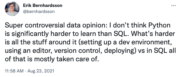
Python has more startup costs. Most SQL interfaces live on a cloud somewhere. Directing a student to a tutorial link that opens a SQL interface with all the data preloaded in the browser is easy. In contrast, to get Python working, you must understand which version you’re working with, how to import (and install) packages like Pandas, access an IDE, and figure out what an IDE is. Web-hosted Jupyter notebooks (like Google Colab) make this a bit easier, but they have their own challenges for a newbie.
Beyond the basic startup cost, there is a lot of information you need to learn before getting into actual data work in Python: data structures like lists and dictionaries, indexing from 0, control structures, etc., not to mention all of Pandas. It is conceptually easier to load into a SQL cloud and get the instruction to type:
SELECT
  DISTINCT(state)
FROM
  payments
Then see a list of all the states associated with customer payments. It makes SQL much more accessible as it quickly builds confidence in a student that they can work with data in code. Importantly, building confidence in a student likely also raises their willingness to keep purchasing courses to pursue their interest in a data career. Not necessarily a bad thing, but it may later be a disappointment when they apply for a data role and find that the application requires them to match charges and payments, and they primarily were only taught how to return aggregate metrics using GROUP BY.
I think it is much better for folks interested in pursuing a data career to learn how to *program* not just how to *code* in Python or SQL. Programming is independent of any specific language and is about thinking algorithmically to solve a problem. It is about designing a solution to solve a problem before implementing it in code using the appropriate data structures for that coding environment.
Often, learning to program and how to code in a language go together as algorithmic solutions are usually implemented as part of the process of designing them. With that in mind, I think it is much better to first learn to code in Python (or another general-purpose language), as this will allow for the development of a broader sense of how to use algorithms and data structures. With these skills, students may have a better chance of securing a data position as a data analyst, engineer, or scientist.
I hope this article has helped you see how to work with payment and charge data. Comparing the fundamental differences in logic between Python and SQL when doing the same task can provide context for aspiring data professionals who may work in these areas.
Resources
Want to Connect?

You can find me @bradchattergoon on Twitter and LinkedIn.