napari: A Multidimensional Image Viewer for Python

A guide to some of the key concepts of napari

napari viewer showing skimage cell3d dataset

What is napari?

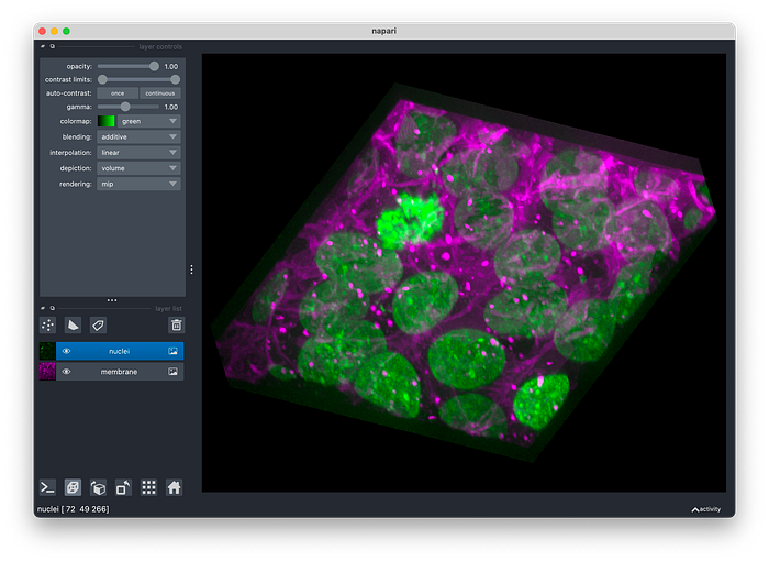
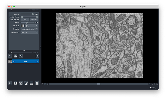
Led by microscopy and Python experts and built by an ever-growing community, napari¹ is an open-source project designed for the browsing, annotating, and analysis of large multidimensional images. napari has quickly become an essential tool to most image analysts due to its high-performance visualisations and its ability to explore a broad range of imaging data, including microscopy, medical imaging, geospatial data, and more.

Why use napari?

napari supports many file and data types, and if a file is not supported natively, then there will almost certainly be a plugin capable of loading it. This leads me to one of the most important aspects of napari, which are the plugins. napari has an incredibly active community with plugins being developed and released almost daily, covering all aspects of image analysis. Furthermore, due to napari being written in Python, it has become particularly attractive to those in the scientific programming community due to the language’s popularity. As it is written in Python, it also opens the doors to integrating its vast ecosystem of machine learning, deep learning, and data science packages. Moreover, by being written in Python, one is able to directly plug into many of the most popular image/data processing Python libraries with examples such as scikit-image², Numpy³, SciPy⁴, and clEsperanto⁵.

How Does napari Work?

One of the key concepts to understand about napari is the idea of layers. Each image you open in the viewer will have its own layer. As such, you’re able to view multiple images or layers at the same time. napari has seven distinct layer types, including Image, Labels, Points, Shapes, Surface, Tracks and Vectors. Each layer corresponds to a different data type, visualisation, and interactivity.

However, I should note that whilst the Image , Labels and Points layers are well developed and ready to use, the Surface , Tracks and Vectors layers are experimental and are still under development. All layers support n-dimensional data and can be quickly visualised and browsed in either 2D or 3D. Lastly, anything present within the viewer is also accessible programmatically via the IPython console, which I’ll explain a bit more about later. Now that we have a rough idea of what napari is, let’s start downloading it!

Installing and Running napari

1. Install Mamba

A simple and recommended way to download most standard Python tools is via Mamba. Briefly, Mamba is a package management system that allows users to download Python or R packages to an environment where they can use them.

Mamba homepage

To install Mamba on Windows, go to this webpage, and download the correct Mambaforge version for your system.

GitHub repository of mini-forge

If you are using Mac or Linux, start by opening the terminal and entering the following command:

curl -L -O "https://github.com/conda-forge/miniforge/releases/latest/download/Mambaforge-$(uname)-$(uname -m).sh"

bash Mambaforge-$(uname)-$(uname -m).sh

Once this completes, Mamba should be installed!

To test that Mamba has been installed correctly, you can open the terminal or command shell and type in the following command:

mamba -V

which will output something like the following if it has been installed correctly:

For more details on Mamba, see these great articles written by Dr. Robert Haase and Mara Lampert at the following links:

• Managing Scientific Python environments using Conda, Mamba, and friends
• Getting started with Mambaforge and Python

2. Creating a Mamba environment

When downloading napari, creating a Mamba environment is generally the best practice. Mamba environments will act as containers for all the Python packages we need to start using napari. To do this, we must first run the following line in the terminal:

mamba create -n napari_env python=3.9

• The mamba keyword calls the Mamba package management system.
• The create keyword tells Mamba we want to create a new environment.
• The -n flag tells Mamba the next statement is the name of the new environment.
• The napari_env declares the name of the new environment.
• The python=3.8 states which version of Python will be installed with the new environment.

This will look like this if the environment has been created correctly.

Once this completes, we then need to activate the environment. This means that when we install the Python packages, all the packages will be installed within the environment and not elsewhere within the computer.

mamba activate napari_env

• The mamba keyword calls the package management system Mamba.
• The activate keyword tells Mamba to activate an environment.
• The napari_env tells Mamba which environment to activate.

Once you’ve done this, the name of the environment will appear in brackets like so:

3. Installing napari

mamba install napari -c conda-forge

• The mamba keyword calls the package management system Mamba.
• The install command is telling Mamba which Python package to install.
• The napari word is the name of the Python package to be installed.
• The -c is declaring which channel to install from.
• The conda-forge is the channel to install napari from.

4. Running napari

If napari has successfully installed, then running it should be as simple as entering the following command in the terminal:

napari

which will open up the following:

The default napari graphical user interface

The napari User Interface

1. Layer controls — This widget will allow you to manipulate specific attributes of a layer. The controls will change depending on what type of layer you have selected. For an image, you can change attributes such as its colormap, opacity, contrast, etc.
2. Delete selected layer — This will delete a selected layer from the Viewer.
3. New labels layer — This will create a new napari Labels layer and add it to the Viewer. The Labels layer allows you to take an array of integers and display each integer as a different random colour with the background colour 0 rendered transparent.
4. New shape layer — This will create a new napari Shapes layer and add it to the Viewer. The Shapes layer allows you to display a list of NxD arrays, each corresponding to one shape.
5. New points layer — This will create a new napari Points and add it to the Viewer. The Points layer allows you to display an NxD array of N points in D coordinates.
6. Layer list — This will show you all the layers you have open in the viewer. You can have multiple layers open at the same time, with each being different layer types, such as Image, Shapes, Labels etc. 6.1) This will allow you to make a layer visible or hide it. 6.2) This icon indicates what type of layer it is.
7. IPython Console — This will show/hide the built-in IPython console, allowing you to programmatically interact with the viewer.
8. Toggle ndisplay — This will change the Viewer to view any visible layers in three dimensions.
9. Change the order of the visible axis — This will transpose a layer across all of its axes.
10. Transpose order of the last two visible axes — This will transpose a layer only across its last two visible axes.
11. Grid mode — This will change the Viewer to show all layers in a grid layout.
12. Reset viewer — This will reset the Viewer to show a layer in its original state. This is especially useful when you’ve scrolled or zoomed so much you don’t know where you are!
13. Scroll bar — If you have a > two-dimensional image, then this will allow you to scroll through each slice of the image.

Running napari from a Python script

To run napari and view an image from a Python script, you must begin by importing napari, then add a loaded image to the viewer with the view_image command. Finally, you can run napari using the napari.run command. Here’s what that looks like:

import napari
from skimage import data

# here we initialise the napari viewer
viewer = napari.Viewer()
# now we're adding the data.cell() image to the viewer
viewer.add_image(data.cell())
# calling napari and telling it begin running
napari.run()

napari viewer showing skimage cell dataset

To load your own local image, it’s a very similar process. Instead of importing the skimage.data sample image, we use the skimage.io.imread, which you pass the file path of your image into, and it will automatically read it and store it into a variable.

import napari
from skimage.io import imread

# reading our image and storing it into the variable img
img = imread('path/to/image.png')
# here we initialise the napari viewer
viewer = napari.Viewer()
# adding the image to the napari viewer
viewer.add_image(img)
# running napari
napari.run()

napari viewer showing EPFL mitochondria dataset

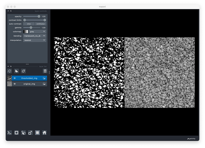
Now, let’s apply a simple threshold to a sample image and view the results in napari. Thresholding can be defined as the process of partitioning an image into a foreground and background. After applying the threshold, we’ll add both the original image and the new threshold image to the viewer.

import napari
from skimage.data import gravel

# creating a variable to store our sample image
original_img = gravel()
# the threshold value to be applied to the image
thresh = 150
# applying the threshold to the image
thresholded_img = original_img > thresh
# creating a napari viewer
viewer = viewer = napari.Viewer()
# adding the original image to the viewer
viewer.add_image(original_img)
# adding our new thresholded image to the viewer
viewer.add_image(thresholded_img)
# running napari
napari.run()

napari viewer showing skimage gravel dataset

As you can see, we’ve applied a threshold to the original image as we now have two layers, the original image, and the threshold image.

We can view them side by side by toggling the grid mode in the blue box, which will give us something like this:

napari viewer showing skimage gravel dataset next to the same image, but after applying a threshold

Plugins for napari

One of the key factors in napari’s popularity recently has been its wide community development of plugins. Plugins are tools that allow developers to customise and extend napari by adding a specific feature. This can include tools used for segmentation to image registration, and the main way of finding such plugins is via the napari hub.

The napari hub is a service of the Chan Zuckerberg Initiative. It’s in collaboration with napari and tries to solve many of the challenges and needs in finding analysis solutions to imaging problems. It allows you to browse the range of plugins being developed by the napari community and offers a brief description of what every plugin does and how to install them.

The napari hub home page

Overview

In this article, we have briefly covered the fundamentals of napari, starting with answering the basic questions of “what is napari,” “why use napari,” and “how does napari work” to running napari from a Python script.

Hopefully, after reading this article, you feel comfortable exploring the ever-growing ecosystem of napari plugins and using napari for your general imaging needs.

Thanks a lot if you have read this far. In the coming months, I will be releasing more articles around napari and general bioimage analysis, so if there are any topics you would like to be covered, don’t hesitate to leave a comment or drop me a message!

Acknowledgement

I’d also like to thank Dr Martin Jones and Dr Robert Haase for their assistance in writing and reviewing this article.

References

1. napari contributors (2019). napari: a multi-dimensional image viewer for Python. doi:10.5281/zenodo.3555620
2. Stéfan van der Walt, Johannes L. Schönberger, Juan Nunez-Iglesias, François Boulogne, Joshua D. Warner, Neil Yager, Emmanuelle Gouillart, Tony Yu and the scikit-image contributors. scikit-image: Image processing in Python. PeerJ 2:e453 (2014) https://doi.org/10.7717/peerj.453
3. Harris, C.R., Millman, K.J., van der Walt, S.J. et al. Array programming with NumPy. Nature 585, 357–362 (2020). DOI: 10.1038/s41586–020–2649–2. (Publisher link).
4. Pauli Virtanen, Ralf Gommers, Travis E. Oliphant, Matt Haberland, Tyler Reddy, David Cournapeau, Evgeni Burovski, Pearu Peterson, Warren Weckesser, Jonathan Bright, Stéfan J. van der Walt, Matthew Brett, Joshua Wilson, K. Jarrod Millman, Nikolay Mayorov, Andrew R. J. Nelson, Eric Jones, Robert Kern, Eric Larson, CJ Carey, İlhan Polat, Yu Feng, Eric W. Moore, Jake VanderPlas, Denis Laxalde, Josef Perktold, Robert Cimrman, Ian Henriksen, E.A. Quintero, Charles R Harris, Anne M. Archibald, Antônio H. Ribeiro, Fabian Pedregosa, Paul van Mulbregt, and SciPy 1.0 Contributors. (2020) SciPy 1.0: Fundamental Algorithms for Scientific Computing in Python. Nature Methods, 17(3), 261–272.
5. Haase, R., Royer, L.A., Steinbach, P. et al. CLIJ: GPU-accelerated image processing for everyone. Nat Methods 17, 5–6 (2020). https://doi.org/10.1038/s41592-019-0650-1