Image Segmentation in Python (Part 2)

Improve model accuracy by removing background from your training data set

Illustration credit: Author

Stuck behind the paywall? Click here to read the full article with my friend link.

Welcome back!

This is the second part of a three part series on image classification. I recommend you to first go through Part 1 of the series if you haven’t already (link below). I’ve gone through the details of setting up the environment and working with image data from Google Drive in Google Colab there. We’ll be using output from that code here.

Introduction to Image Augmentation in Python

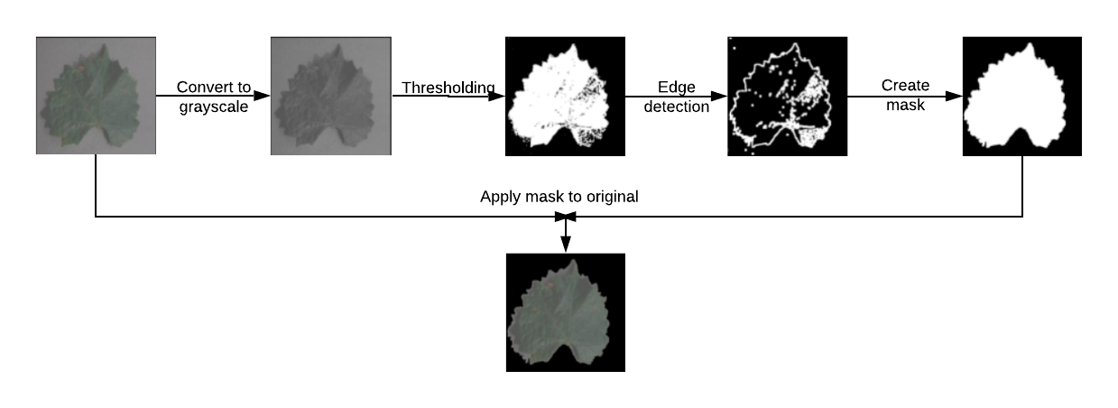
Image segmentation is the process of “partitioning a digital image into multiple segments”. Since we are just concerned about background removal here, we will just be dividing the images into the foreground and the background.

This consists of five basic steps:

1. Convert the image to grayscale.
2. Apply thresholding to the image.
3. Find the image contours (edges).
4. Create a mask using the largest contour.
5. Apply the mask on the original image to remove the background.

I’ll be explaining and coding each step. Onward!

Setting Up the Workspace

If you have gone through Part I and have executed the code till the end, you can skip this section.

For those who haven’t, and are here just to learn image segmentation, I’m assuming that you know how Colab works. In case you don’t please go through Part I.

The data set is available here. This is the result of the code from Part I. Open the link while signed in to your Google account so that it’s available in the “Shared with me” folder of your Google Drive. Then open Google Colab, connect to a runtime, and mount your Google Drive to it:

Follow the URL, select the Google account which you used to access the data-set, and grant Colab permissions to your Drive. Paste the authorization code at the text box in the cell output and you’ll get the message Mounted at /gdrive.

Then we import all the necessary libraries:

import cv2
import glob
import matplotlib.pyplot as plt
import numpy as np
from PIL import Image
import random
from tqdm.notebook import tqdm
np.random.seed(1)

Our notebook is now set up!

Reading Images from Drive

If you’re using data from the link shared in this article, the path for you will be ‘/gdrive/Shared with me/LeafImages/color/Grape*/*.JPG’.

Those who followed Part I and used the entire training set should see 4062 paths.

Next we load the images from the paths and save them to a NumPy array:

A shape of (20, 256, 256, 3) signifies that we have 20 256x256 sized images, with three color channels.

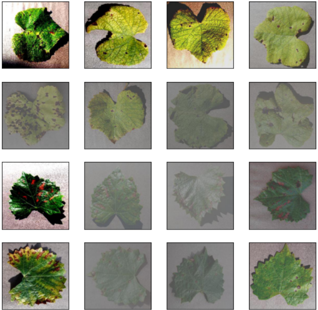
Let’s see how these images look:

plt.figure(figsize=(9,9))
for i, img in enumerate(orig[0:16]):
    plt.subplot(4,4,i+1)
    plt.xticks([])
    plt.yticks([])
    plt.grid(False)
    plt.imshow(img)
plt.suptitle("Original", fontsize=20)
plt.show()

Original Images

Grayscaling

The first step in segmenting is converting the images to grayscale. Grayscaling is the process of removing colors from an image and representing each pixel only by its intensity, with 0 being black and 255 being white.

OpenCV makes this easy:

We can see from the shape that the color channels have been removed.

Display the converted images:

plt.figure(figsize=(9,9))
for i, img in enumerate(gray[0:16]):
    plt.subplot(4,4,i+1)
    plt.xticks([])
    plt.yticks([])
    plt.grid(False)
    plt.imshow(cv2.cvtColor(img, cv2.COLOR_GRAY2RGB))
plt.suptitle("Grayscale", fontsize=20)
plt.show()

Grayscale images

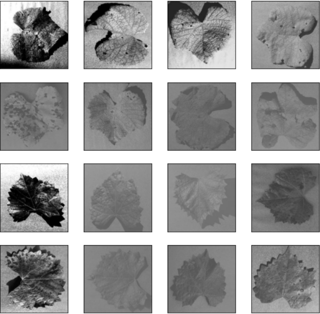
In the first image, we can see that the first pixel (top-left) is white, while the ones at the bottom-left are black. This can be verified by checking the pixel array for the first image:

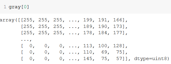
Indeed, the pixels at the top left are white (255), and the ones at the bottom-left are black (0).

Thresholding

In image processing, thresholding is the process of creating a binary image from a grayscale image. A binary image is one whose pixels can have only two values — 0 (black) or 255 (white).

In the simplest case of thresholding, you select a value as a threshold and any pixel above this value becomes white (255), while any below becomes black (0). Check out the OpenCV documentation for image thresholding for more types and the parameters involved.

thresh = [cv2.threshold(img, np.mean(img), 255, cv2.THRESH_BINARY_INV)[1] for img in tqdm(gray)]

The first parameter passed to cv2.threshold() is the grayscale image to be converted, the second is the threshold value, the third is the value which will be assigned to the pixel if it crosses the threshold, and finally we have the type of thresholding.

cv2.threshold() returns two values, the first being an optimal threshold calculated automatically if you use cv2.THRESH_OTSU, and the second being the actual thresholded object. Since we’re only concerned about the object, we subscript [1] to append only the second returned value in our thresh list.

You can choose a static threshold, but then it won’t be able to take the different lighting conditions of different photos into account. I’ve chosen np.mean(), which gives the average value of a pixel for the image. Lighter images will have a value greater than 127.5 (255/2), while darker images will have a lower value. This lets you threshold images based on their lighting conditions.

For the first image, the threshold is 126.34, which means that the image is slightly darker than average. Any pixel which has a value greater than this will be converted to white, and any less, will be made black. But wait! If you notice the grayscale image, the leaf is darker than the background. If we apply a normal threshold, the darker pixels become black, while lighter pixels become white. This will apply a black mask on the leaf, not the background. To deal with this, we use the THRESH_BINARY_INV method, which inverts the thresholding process. Now, pixels having an intensity greater than the threshold will be made black — those with less, white.

Lets have a look at the pixel intensities for the first thresholded image:

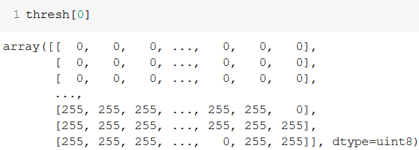
As you can see, the pixels which were lighter (top row) in the grayscale array are now black, while those which were darker (bottom row), are now white.

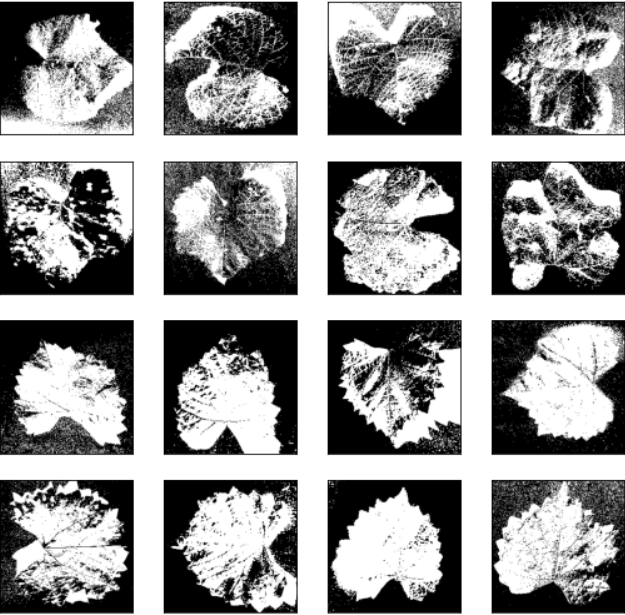
Lets see the thresholded images to verify:

Edge Detection

Edge detection, as the name suggests, is the process of finding boundaries (edges) of objects within an image. In out case, it will be the boundary between the white and black pixels.

OpenCV lets you implement this using the Canny algorithm.

edges = [cv2.dilate(cv2.Canny(img, 0, 255), None) for img in tqdm(thresh)]

Dilate is a noise removal technique which helps in joining broken parts of an edge together, so that they form a continuous contour. Read more about some other noise removal techniques in edge detection here. You can also experiment with them and see if the results look better.

0 and 255 here are the lower and upper threshold values respectively. You can read about their use in the documentation. In our case, since the images are already thresholded, these values don’t really matter.

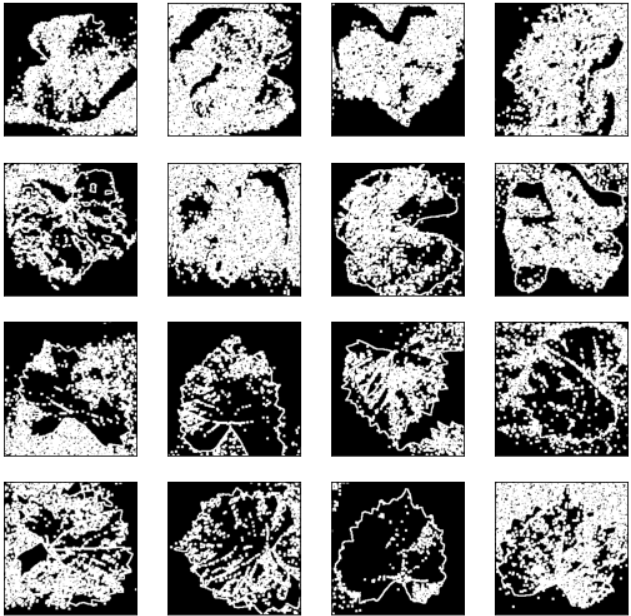
Lets plot the edges:

plt.figure(figsize=(9,9))
for i, edge in enumerate(edges[0:16]):
    plt.subplot(4,4,i+1)
    plt.xticks([])
    plt.yticks([])
    plt.grid(False)
    plt.imshow(cv2.cvtColor(edge, cv2.COLOR_GRAY2RGB))
plt.suptitle("Edges", fontsize=20)
plt.show()

Edge detection

Masking and Segmenting

Here at last. This involves quite a few steps, so I’ll be taking a break from list comprehensions for easy comprehension.

Masking is the process of creating a mask from an image to be applied to another. We take the mask and apply it on the original image to get the final segmented image.

We want to mask out the background from our images. For this, we first need to find the edges (already done), and then find the largest contour by area. The assumption is that this will be the edge of the foreground object.

cnt = sorted(cv2.findContours(img, cv2.RETR_LIST, cv2.CHAIN_APPROX_SIMPLE)[-2], key=cv2.contourArea)[-1]

This is already a handful — let’s dissect!

First we find all the contours cv2.findContours(img, cv2.RETR_LIST, cv2.CHAIN_APPROX_SIMPLE). The documentation is your friend again if you want to get into the details of the second and third parameters. This returns the image, the contours, and the contour hierarchy. Since we want only the contour, we subscript it with [-2] to retrive the second last returned item. Since we have to find the contour with the largest area, we wrap the entire function within sorted(), and use cv2.contourArea as the key. Since sorted sorts in ascending order by default, we pick the last item with [-1] which gives us the largest contour.

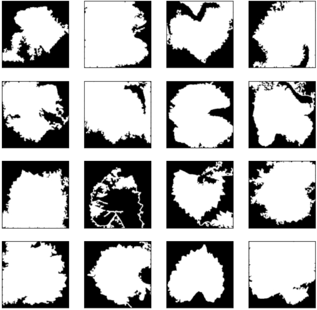
Then we create a black canvas of the same size as our images mask = np.zeros((256,256), np.uint8). I call this “mask” as this will be the mask after the foreground has been removed from it.

To vizualise this, we merge the largest contour on the mask, and fill it with white cv2.drawContours(mask, [cnt], -1, 255, -1)). The third parameter ,-1 in our case, is the number of contours to draw. Since we have already selected just the largest contour, you can use either 1 or -1 (for all) here. The second parameter is the fill color. Since we have a single channel and want to fill with white, it is 255. Last is the thickness.

Since a picture is worth a thousand words, let the below hastily made illustration make the process a bit simpler to understand:

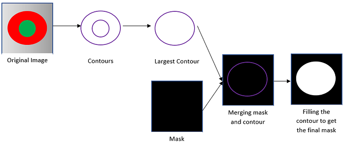
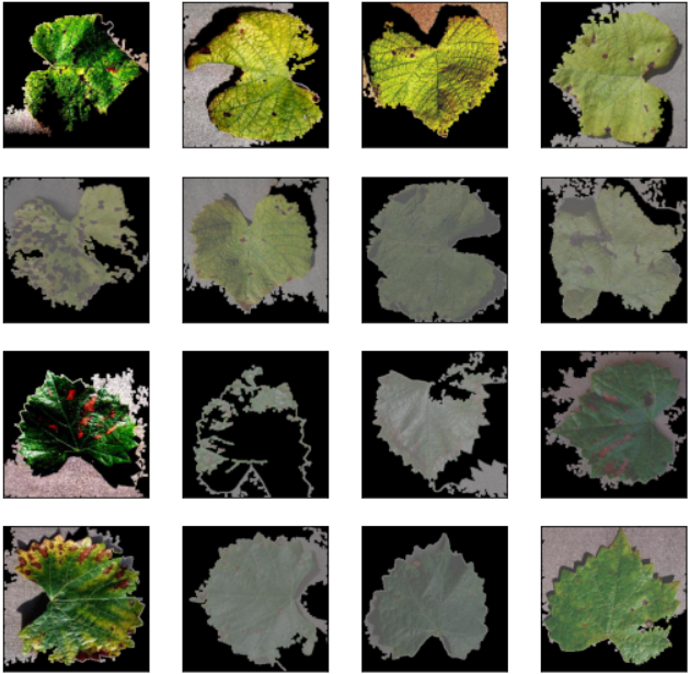
I think you can guess the final step — superimposing the final mask on the original image to effectively remove the background.

This can be done using the bitwise_and operation. This tutorial will help you to understand how that actually works.

dst = cv2.bitwise_and(orig, orig, mask=mask)

Now we just wrap this section inside a loop to append all the masks and segmented images to their respective arrays, so we can finally see what our work looks like:

masked = []
segmented = []
for i, img in tqdm(enumerate(edges)):
    cnt = sorted(cv2.findContours(img, cv2.RETR_LIST, cv2.CHAIN_APPROX_SIMPLE)[-2], key=cv2.contourArea)[-1]
    mask = np.zeros((256,256), np.uint8)
    masked.append(cv2.drawContours(mask, [cnt],-1, 255, -1))
    dst = cv2.bitwise_and(orig[i], orig[i], mask=mask)
    segmented.append(cv2.cvtColor(dst, cv2.COLOR_BGR2RGB))

Plotting the masks:

plt.figure(figsize=(9,9))
for i, maskimg in enumerate(masked[0:16]):
    plt.subplot(4,4,i+1)
    plt.xticks([])
    plt.yticks([])
    plt.grid(False)
    plt.imshow(maskimg, cmap='gray')
plt.suptitle("Mask", fontsize=20)
plt.show()

Masks

And the final segmented images:

plt.figure(figsize=(9,9))
for i, segimg in enumerate(segmented[0:16]):
    plt.subplot(4,4,i+1)
    plt.xticks([])
    plt.yticks([])
    plt.grid(False)
    plt.imshow(cv2.cvtColor(segimg, cv2.COLOR_BGR2RGB))
plt.suptitle("Segmented", fontsize=20)
plt.show()

Segmented images

We can then finally these images in a separate “segmented” folder:

import os
for i, image in tqdm(enumerate(segmented)):
    directory = paths[i].rsplit('/', 3)[0] + '/segmented/' + paths[i].rsplit('/', 2)[1]+ '/'
    os.makedirs(directory, exist_ok = True)
    cv2.imwrite(directory + paths[i].rsplit('/', 2)[2], image)

Expecting Better Results?

This was just an introduction to the process — we didn’t delve too deeply into the parameters so the results are far from perfect. Try to figure out which step introduced distortion and think of how you can improve this step. As I said earlier, the OpenCV Image Processing tutorial is a great place to start.

Grayscale > Threshold > Edge > Mask

I would love to see your results in the comments and learn how you achieved them!

Stay Tuned…

You can find the Colab notebook I used here.

This concludes the second part of the trilogy. Stay tuned for the final part where we use these segmented images to train a very basic image classifier. The link to it will be added here once published.

Thanks for reading, bouquets, and brickbats welcome!

Medium still does not support payouts to authors based out of India. If you like my content, you can buy me a coffee :)

Siddhant Sadangi is creating python web-apps on Streamlit