Build a NoSQL Database From Scratch in 1000 Lines of Code

Introducing LibraDB, a working database I created using Go

Photo by Pixabay

Chapter 1

I’m a fan of personal projects. Throughout the years, I have had the pleasure of writing multiple database-related blogs/GitHub projects. Now, I’ve decided I want one project to rule them all!

I’ve implemented my database in Go and decided to share my knowledge by writing a blog post describing all the steps. This post is quite long, so I originally it was meant to be a 7 parts series. Eventually, I decided to keep it into one long blog post that is split into 7 original parts. This way, you stop and easily come back to each chapter.

The database is intentionally simple and minimal, so the most important features will fit in but still make the code short.

The code is in Go, but it’s not complicated, and programmers unfamiliar with it can understand it. If you do know Go, I encourage you to work along!

The entire codebase is on GitHub, and there are also around 50 tests to run when you’re done. In a second repo, the code is split into the 7 logical parts, each part in a different folder.

We will create a simple NoSQL database in Go. I’ll present the concepts of databases and how to use them to create a NoSQL key/value database from scratch in Go. We will answer questions such as:

• What is NoSQL?
• How to store data on disk?
• The difference between disk-based and in-memory databases
• How are indexes made?
• What is ACID, and how do transactions work?
• How are databases designed for optimal performance?

The first part will start with an overview of the concepts we will use in our database and then implement a basic mechanism for writing to the disk.

SQL vs NoSQL

Databases fall into different categories. Those that are relevant to us are Relational databases (SQL), key-value store, and document store (Those are considered NoSQL). The most prominent difference is the data model used by the database.

Relational databases organize data into tables (or “relations”) of columns and rows, with a unique key identifying each row. The rows represent instances of an entity (such as a “shop” for example), and the columns represent values attributed to that instance (such as “income” or “expanses”).

In relational databases, business logic may spread across the database. In other words, parts of a single object may appear in different tables across the database. We may have different tables for income and expenses, so to retrieve the entire shop entity from the database, we would have to query both tables.

Key-value and document stores are different. All information of a single entity is saved collectively in collections/buckets. Taking the example from earlier, a shop entity contains both income and expenses in a single instance and resides inside the shops collection.

Document stores are a subclass of key-value stores. In a key-value store, the data is considered inherently opaque to the database, whereas a document-oriented system relies on the document’s internal structure.
For example, in a document store, it’s possible to query all shops by an internal field such as incomes, whereas key-value could fetch shops only by their id.

Those are the basic differences, though, in practice, there are more database types and more reasons to prefer one over another.

Our database will be a key-value store (not a document store) as its implementation is the easiest and most straightforward.

Disk-Based Storage

Databases organize their data (collections, documents …) in database pages. Pages are the smallest unit of data exchanged by the database and the disk. It’s convenient to have a unit of work of fixed size. Also, it makes sense to put related data in proximity so it can be fetched all at once.

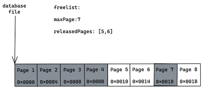
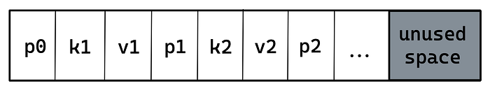
Database pages are stored contiguously on the disk to minimize disk seeks. Continuing our earlier example, consider a collection of 8 shops, where a single page is occupied by 2 shops. On the disk, it’ll look like the following:

MySQL has a default page size of 16Kb, Postgres page size is 8Kb, and Apache Derby has a page size of 4Kb.

Bigger page sizes lead to better performance, but they risk having torn pages. A scenario where the system crashes in the middle of writing multiple database pages of a single write transaction.

Those factors are considered when choosing the page size in a real-life database. Those considerations are not relevant to our database, so we will arbitrarily choose the size of our database pages to be 4KB.

Underlying Data Structure

As explained, databases store their internal data across many pages, which are stored on the disk. Databases employ data structures to manage the quantity of pages.

Databases use different data structures to organize pages on the disk, mostly B/B+ Trees and hash buckets. Each data structure has its own benefits and merits: read/write performance, support for more complex queries such as sorting or range scans, ease of implementation, and many more.

We will use B-tree since it allows for easy implementation, but its principles are close to what is used in real-world databases.

Our Database

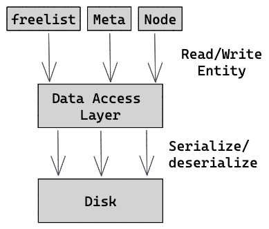
Our database will be a key-value store. Its underlying data structure is a B-Tree, and the size of each page is 4KB. It’ll have the following architecture:

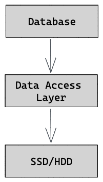
Database manages our program and is responsible for orchestrating transactions — those are sequences of read and write operations. It also faces the programmers using the database, and serves their requests.

Data Access Layer (DAL) handles all disk operations and how data is organized on the disk. It’s responsible for managing the underlying data structure, writing the database pages to the disk, and reclaiming free pages to avoid fragmentation.

Start Coding

We will build our database from the bottom-up, starting from the Data Access Layer (DAL) component. We’ll begin coding by creating a file for it. We’ll have a struct, a constructor, and a close method.

Database Pages

Reading and writing database pages will be managed by the DAL. We’ll add a struct for the page type inside dal.go. It'll contain a number that serves as a unique ID, but it’s serves a bigger role. That number is used to access the page with pointer arithmetic like (PageSize*pageNum). We'll also add PageSize attribute to dal .

Finally, we’ll add a constructor and read and write operations for it. Notice how, on lines 12 and 25, the correct offset in the file is calculated given the page size and the page number.

Freelist

Managing pages is a complex task. We need to know which pages are free and which are occupied. Pages can also be freed if they become empty, so we need to reclaim them for future use to avoid Fragmentation.

All this logic is managed by the freelist. This component is part of the DAL. It has a counter named maxPage holding the highest page number allocated so far, and an attribute called releasedPages for tracking released pages.

When allocating a new page, releasedPages is assessed first for a free page. If the list is empty, the counter is incremented, and a new page is given, increasing the file size.

Occupied pages are in grey. The free pages are in white.

We will start by creating the file freelist.go, defining the type for freelist , and adding a constructor newFreeList. Then, we need to add getNextPage and releasePage . Our database uses the first page for storing metadata (which will be explained in the next chapter), so we can only allocate new pages with numbers greater than 0.

Finally, we will embed the freelist inside our dal structure and create an instance when opening the database.

Chapter 1 Conclusion

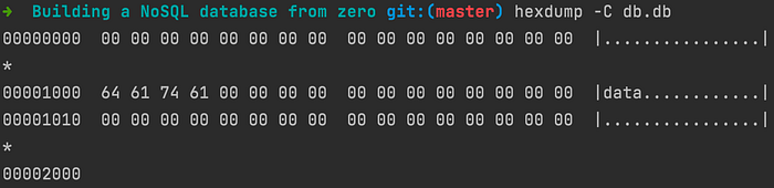
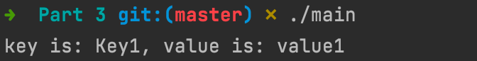
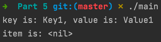
So far, our database supports reading and writing pages. To test our work, we can create a main function, write a page and look at how data is stored.

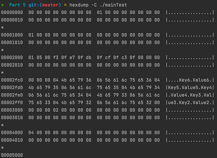
The command hexdump , together with the -C flag is used for displaying the contents of a binary file.

The first 4096 bytes (1000 in hex as seen on the left) are reserved for the metadata, and our data is right after it.

Our database is functioning as long as the program is running. If the program is killed, we can’t know which pages are empty and which contain actual data. To start, it means the freelist needs to be persisted to the disk. This will be our topic for the next chapter.

You can check here a complete version of this part’s code.

Chapter 2

We continue building our database. In the last chapter, we looked at the general architecture of our database.

Then we implemented the Data Access Layer that handles disk operations. So far, it supports: opening and closing the database file, writing and reading data into disk pages, and also managing empty and occupied pages using the freelist .

In this chapter, we will implement persistence to disk. It’s essential to save the database state to the disk so it can operate correctly between restarts. The DAL will be responsible for it.

We will start by committing the state of the freelist to the disk.

Start Coding

To save the state of freelist we want to write it as a database page to the disk. It’s common in databases to have a page holding metadata about the database.

It can be page numbers of essential pages- freelist in our case. It can also hold the magic number- a constant numerical or text value used to identify the file format (we will meet it in the last chapter). In our case, it’ll be both.

To track the freelist page number, we will add a new page called meta . It’s a special page since it’s fixed and located on number 0. This way, upon a restart, we can read the meta page from page number 0 and follow it to load the freelist content.

Meta Page Persistence

A typical pattern in our database is defining serialize and deserialize methods for converting an entity into raw data that fits a single page. And wrapping those with reading and writing methods that return the entity itself.

We will create a new file named meta.go , define a new type meta and a constructor.

We need to serialize meta to []byte so we can write it to the disk. Unfortunately, Go does not support an easy conversion of structs to binary the way C does without using the Unsafe package (which we won’t use for obvious reasons), so we’ll have to implement it ourselves.

In each method, we’ll have a position variable (pos) for tracking the position in the buffer. It’s similar to the cursor in files.

We will also create a new file const.go for holding the sizes and declare a new constant pageNumSize. It contains the size of a page number (in bytes).

The const.go file answers the how many bytes to store for each variable, and the serialize and deserialize take care of where to keep it inside the page.

Finally, we’ll add the methods writeMeta and readMeta using the previous meta serialize/deserialize and read/write page methods.

Freelist Persistence

We have defined the meta page so we know where to find the freelist data. Now, we need to add methods for reading/writing the freelist itself. As before, we’ll add methods for serializing and deserializing.

Next, we’ll embed the meta inside the dal struct.

Add methods for reading and writing a freelist page using the page number located inside the meta struct.

And finally, update the dal constructor to check for the database’s existence. If it doesn’t, a new meta file is created, and the freelist and meta pages are initialized. If it does, read the meta page to find the freelist page number and deserialize it.

Chapter 2 Conclusion

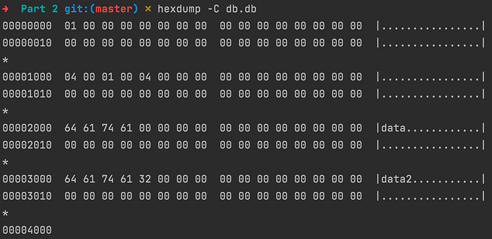
Ok! We have persistence. We can play around by creating a new database, closing it, and then opening it again.

Notice the meta page on page 0 (starting at line 1) containing the number 1 of the freelist page.

Right below (third line) is the freelist . We have 4, 1, 4. The first 4 indicate the maximum allocated page number. 1 shows the length of the released pages list, and the last 4 account for the only released page.

And finally, we have our data, and as you can see in the right column, it behaves correctly after the DB restarts.

In the next episode, we’ll start exploring B-Trees which are the main star of the database. It’ll take us a few episodes to cover it completely. We’ll talk about how they help us in organizing the data and how to store them on disk.

You can check here a complete version of this part’s code.

Chapter 3

We finished persisting our database on the disk in the last two chapters. It means our database can restore its previous state between restarts. It also supports reading and writing pages to the disk, but we have to take care of the bookkeeping of the data. In other words, when fetching an item from the database, we must remember where it was inserted.

Today, we will talk about B-Trees, the database’s main star. We will see how they help us organize the data, so the user doesn’t have to track where each object is located on the disk.

Binary Search Tree

A binary search tree (also called BST) is a data structure used for storing data in an ordered way. Each node in the tree is identified by a key, a value associated with this key, and two pointers (hence the name binary) for the child nodes. The invariant states that the left child node must be less than its direct parent, and the right child node must be greater than its immediate parent.

Binary Search Tree

This way, we can easily find elements by looking at each node’s value and descent accordingly. If the searched value is smaller than the current value, descend to the left child; if it’s greater, descend to the right.

A binary search tree allows for fast lookup, addition, and removal of data items since the nodes in a BST are laid out so that each comparison skips about half of the remaining tree.

Motivation

Why do we even need a tree in the first place? A straightforward approach would be to create a text file and write data sequentially. Writing is fast, as new data is appended to the end of the file. On the other hand, reading a specific item requires searching the entire file. If our file gets big, reading will take a long time.

Obviously, it’s not suited for many real-life applications. Compared to the previous approach, BST offers slower writing in favor of better reading. This balanced approach is ideal for general-use databases.

Another consideration is disk access. It is costly, so it has to be kept to a minimum when designing a data structure that resides on the disk.

A binary tree node has 2 children, so having 2⁵=32 items, for example, will result in a tree with 5 levels. Searching for an item in the tree will require descending 5 levels in the worst case and, in turn, 5 disk accesses for each level. 5 is not much, but can we do better?

B-Tree

B-Tree is a generalization of a binary search tree, allowing for nodes with more than two children. Each node has between k to 2k key-value pairs and k+1 to 2k+1 child pointers, except the root node with as few as 2 children.

By having more children in each node, the tree’s height gets smaller, thus requiring fewer disk accesses.

K-V indicates a key-value pair. P indicates a child pointer

Coding

We will start by creating a new file node.go and defining new types for Node for a B-Tree node and Item representing a key-value pair.

We will also add isLeaf and a constructor for Node and Item.

Node Page Structure

We want to store Node contents on the disk. A trivial approach would be a concatenation of “key-value-child pointer” triplets, but it has a significant downside.

Items contain keys and values of different sizes. It means iterating over key-value pairs becomes a non-trivial task since we can’t know how many bytes the cursor should advance each iteration.

pages are denoted by p, keys by k, and values by v

To solve that problem, we will use a technique called slotted pages. The page is divided into two memory regions. At end of the page lie the keys and values, whereas at the beginning are fixed size offsets to the records.

We will also add a header containing the number of records in the page and a flag indicating if the page is a leaf (As leaves don’t have child pointers).

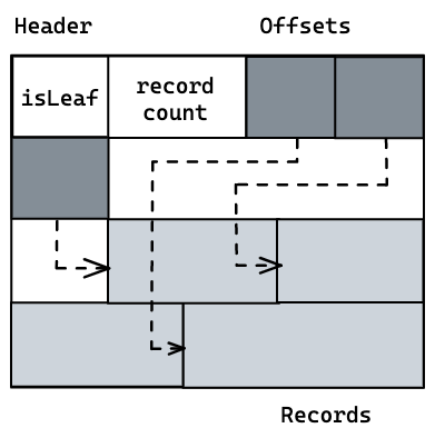
This design allows making changes to the page with minimal effort. The logical order is kept by sorting cell offsets, so the data doesn’t have to be relocated.

Each node is serialized to a single page, but It’s important to understand the distinction between the two.

Node contains only key-value pairs, and it’s used at a higher level. Page on the other hand, works on the storage level and holds any type of data, as long as it’s 4KB in size. It can contain the key-value pairs organized in a slotted page structure, but also freelist and meta which are laid in a less strict form.

Nodes Persistence

As we’ve done in previous chapters, we will add the serialization and deserialization of the database node. Those methods convert data from/to a slotted page format.

The implementation is lengthy and technical, and there’s nothing new to the details above. It’s better to focus general design described above than the implementation itself (Although I encourage you to read the code).

We will also add getNode , writeNode and deleteNode for returning a node.
The first two methods return the node struct itself so they are the same as what we did with freelist and meta .

deleteNode signals to the freelist that a node can be deleted, so its page id can be marked as released.

Search, Insert, and Delete

Before implementing the algorithms for search, insert and delete, it’s safe to assume we will make many calls to receive and write nodes.
We will wrap the calls to the dal with a layer of our own. In future parts, this will come in handy.

Search

Searching a B-Tree is done using a binary search. The algorithm starts with the root node and traverses all the keys until it finds the first key greater than the searched value. Then, we descend toward the relevant subtree using the corresponding child pointer and repeat the process until the value is found.

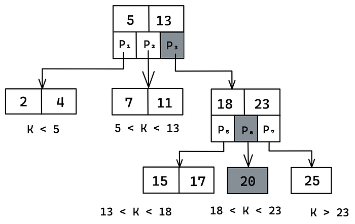
In the example, 20 is supplied. In the first level, no keys match 20 exactly, so the algorithm descends into the correct range- all the numbers bigger than 13. The process is repeated on the rightmost node in the second level

The function findKeyInNode searches for a key inside a node, as in the figure above. It compares searched key with the keys in each level. If a match is found, then the function returns. If the key doesn’t exist, then the correct range is returned.

Now we want to traverse the entire tree and use the previous function when searching each node. We will perform a search similar to a binary search. The only difference is that searching is performed with many children and not two, as described in the image above.

The findKey function is a wrapper around findKeyHelper where the heavy lifting is performed.

As explained, searching is done recursively from a given node, usually the root. Every node can be reached from its parent, but since the root has no parents, we reach it by saving its page number inside the meta page.

The root attribute was added to the meta struct, and serialize and deserialize were to handle this field as well.

Chapter 3 Conclusion

Let’s test our search method. Our DB performs a search in a B-Tree, so it expects the database pages to be laid in a B-tree format.

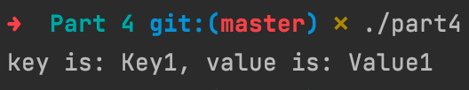
We don’t have a way to create one yet, so I’ve added a mock file named mainTest that is already built this way. This file contains a key-value pair. The key is “Key1” and the value “Value1”.

In the next two chapters, we will implement writing and deleting from the database. You can find the code of this part here.

Chapter 4

In the last chapter, we talked about B-Trees. They are a binary search tree generalization, allowing for nodes with more than two children. Tree height was minimized, thus reducing disk access.

We also talked about slotted pages. A layout for organizing key-value pairs of different sizes by positioning fixed-sized offsets at the beginning and the actual data itself at the end.

Finally, we started implementing basic operations on B-Trees: Search, Insertion, Delete. In the previous chapter, we implemented the search operation. We will do the insertion in this one.

Problem

Inserting new items might cause a node to have too many items. For example, when all the new pairs get inserted into the same node.

It makes operations slower as we iterate over more items every time the node has to be accessed. Apart from that, it leads to a more severe problem. Nodes are translated to fixed-size database pages, so there’s a limitation on the amount of key-value pairs in each node based on the total size of the key-value pairs.

Deletion suffers a similar problem. Deleting key-value pairs from the same node can shrink a node, so it contains very few key-value pairs. At this point, it’s better to reallocate those pairs into a different node someway.

To know if a node has reached maximum or under-occupancy, we must define it first. We will add an upper and lower threshold, a percentage of the page size.

In the code, we introduce Options, that will be initialized by the user and used inside our DB init function.

We will also add new methods to dal and node for calculating a node size in bytes and comparing it to the thresholds. elementSize calculates the size of a single key-value-child triplet at a given index. nodeSize sums the node header size and the sizes of all the keys, values, and child nodes.

Solution

When a node in the tree suffers from too many key-value pairs, the solution is to split it into two nodes.

Splitting is done by allocating a new node, transferring half of the key-value pairs there, and adding its first key and a pointer to that node to the parent node. If it’s a non-leaf node, then all the child pointers after the splitting point will also be moved.

The first key and a corresponding pointer are moved to the parent, thus increasing its occupancy. The process might result in overflow, so rebalancing must be repeated recursively up the tree.

Splitting is done when inserting 4 and 7. Image taken from Wikipedia

Insertion

The algorithm for insertion of an item goes as follows:

1. Search the tree to find the leaf node where the new element should be inserted and add it.
2. If the node is over maximum occupancy, rebalance the tree as described above:
   a. Find the split index
   b. Values less than the separation value are left in the existing node and values greater than the separation value are put into a newly created right node.
   c. The separation value is inserted in the node’s parent.
3. Repeat step 2, starting from the insertion node to the root.

Auxiliary methods

We will start with step 1 of the algorithm. The method addItem adds a key-value pair at a given index and then shifts all the pairs and children. This trivial method could have been easily shipped with the standard library.

For step 2, we will add four methods to determine if a node reached maximum occupancy. (or minimum occupancy which is needed for the delete)

We will add corresponding methods to node for decoupling, which will aid us later.

Now that we know if a rebalance has to occur, we will write the rebalancing itself. Focusing on 2.a, getSplitIndex calculates the index where the node should be split based on the element size and the minimum node size. It sums the sizes of key-value pairs in bytes. Once enough is accumulated, the index is returned.

Finally, we are going to add split to handle steps 2.b and 2.c .It is called on a node and receives one of its child nodes and its index in the childNodes list.

As explained earlier, the split index is determined first. The pairs to the left of the split index are untouched, whereas the pairs to the right are moved to a new node. If child pointers exist, the second half is moved as well.

The pair in the split index is moved to the parent, and a pointer to the newly created node is added at the correct position in the parent.

Put it all together

Before we combine the methods above to an insert function, we will introduce the concept of a collection. A collection is a grouping of key-value pairs. A collection is the equivalent of an RDBMS table. Key-value pairs in a collection have a similar purpose.

We will return to the concept of collections in later articles. For now, we will add a struct called Collection and the Find and Put methods.

A collection is B-Tree on its own. So each collection has a name and a root page marking the tree root node.

The Find method loads the collection root node and performs findKey on that node to locate the key. If a key wasn’t found, nil is returned.

The Put sums all the work we’ve done in this chapter. It receives a key-value pair from the user and inserts it into the collection’s B-Tree.

On lines 9–23, the method checks if a root node was already initialized or its first insertion, so a new root has to be created.

On lines 26–36, we search the tree where insertion should occur. findKey returns the node and the index where insertion should happen. It also returns nodes (as indexes - each node can be retrieved from its parent childNodes array) in the path leading to the modified node if we need to rebalance the tree.

On lines 31–41, we perform the actual insertion. We first check if the key already exists. If so, we only override it with the new value. If it doesn’t, we insert it. Due to how B-Tree works, new items can be added only to leaf nodes. It means we don’t need to care for children.

Finally, we rebalance on lines 49–56 and 59–71 if needed. The first block rebalances up the insertion path, excluding the root. The second block rebalances the root and updates the collection’s root pointer.

Chapter 4 Conclusion

This part was focused on insertion into the database. Now we can insert and find items in the database as the user would have done.

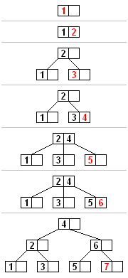
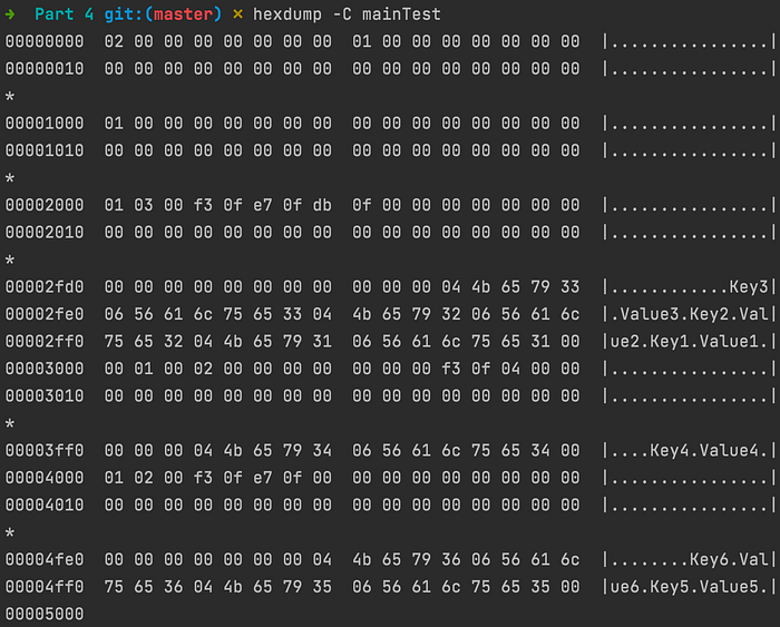
In the code below, we’re creating a new database with MinFillPercent and MaxFillPercent that will cause a node to split when a node has six items or more. We create a new collection assigning the DB root page as the collection root page. Finally, we simulate an actual user operation of adding new items to a collection and searching for them.

Running hexdump on our file, we can observe a split has occurred. We have a root node containing 4. Then we have two children nodes, one with the pairs 1–3 and another node with keys 5–6.

Also, since nodes are designed as slotted pages, observe how the upper and lower addresses are written on each page, and the space in between remains empty.

In the next part, we will focus on deleting. It’ll be less intensive than this part as many of the functions we’ve added in this part will be used later.

You can check the code for this part here.

Chapter 5

We discussed B-Trees and implemented Find and Insert methods in the last two parts. In this part, we will implement the Delete operation and finish discussing B-Trees.

Deletion

The algorithm for deleting an item goes as follows:

1. Locate the item for deletion.
2. Delete the item:
   a If the value is in a leaf node, simply delete it from the node.
   b Otherwise, (the value is in an internal node), choose a new separator — the largest element in the left subtree, remove it from the leaf node it is in, and replace the element to be deleted with the new separator
3. Rebalance the tree, starting from the leaf node or the node the separator was chosen from according to the case above.

Deletion Implementation

We will focus on point 2.

We have two scenarios we need to handle. The first (2.a) is to delete a node from a leaf node. This case is trivial since we only need to remove it from the node.

If, on the other hand, we encounter an internal node (2.b), we need to locate its predecessor and make it the new separator. On line 15, we choose the left subtree and descend in lines 20–27 to the rightmost child, giving us the node with the biggest items in the left subtree.

On lines 30–32, we replace the item to be deleted with its predecessor- the rightmost pair in the left subtree and remove it from the leaf node it was in.

Rebalance

We will focus on point 3.

When entering a new item to a node, it might lead to an overflow in one of the nodes causing the tree to get out of balance. Deletion can cause underflow, so we would have to rebalance the tree right after.

Unlike insertion, where rebalancing is done only by splitting a node, rebalancing after a delete operation can be either merging or rotating nodes.

Rotation can be done to the right or the left, depending on which node has an item to spare. A right rotation, for example, is done by copying the separator key from the parent to the start of the underflow node and replacing the separator key with the last element of its left sibling. When rotating a non-leaf node, the last child pointer of the left sibling is moved to the start of the unbalanced one. A similar approach is made when performing a left rotation.

In the example below, 15 is deleted causing the right child to have too few items. This results in a right rotation.

Right rotation

If no sibling can spare an element, the deficient node must be merged with a sibling. The merge causes the parent to lose a separator element, so the parent may become deficient and need rebalancing. Rebalancing may continue all the way to the root.

In this case, 15 is deleted. A right rotation can’t be performed as will it leave the left child in a deficit. Therefore, the solution is to merge the nodes to a single node.

Merge

Similarly to the previous chapter, we will start adding some auxiliary functions and combine them into a single function under the collection struct.

Our first two functions are right and left rotation. The functions are almost identical so let’s examine rotation to the right.

Rotation is done as explained in the comments. Given node A, we remove its last item. We replace it with the item in the correct index in the parent node and take the item originally in the parent, putting it in the B node.

The correct index is the index of the item between those two nodes in the parent. If any child pointers exist, they are moved as well.

The code for both rotations is similar. The differences are the affected nodes and the key-value pairs being moved.

Next, is merge. The merge function receives a node and its index. Then, it merges that node with its left sibling, transferring its key-value pairs and child pointers. After the function finishes, it deletes the node.

Finally, we will write reblanceRemove that determines what algorithm should be applied when the tree gets out of balance.

In each rotation (lines 9–19 and 22–32), we ensure the unbalanced node is not on the edge, so it has a left/right sibling. We also ensure that the sibling can spare an element, meaning its sibling won’t be underflow after the operation. If both conditions are true, rotation is chosen.

If both conditions don’t hold, then we perform a merge (lines 36–45). The merge function merges a node with its left sibling. If we are on the leftmost sibling, use one node to the right, hence the if condition on line 36.

Putt it all together

We will add a new method Remove to collection. On lines 8–11, the root node is loaded, then on 13–16, we perform step 1 in our algorithm of locating the item to delete. If it doesn't exist, we return in lines 18–20.

On lines 22–30, we delete the item according to step 2 in the algorithm. We extend our ancestor list to track any nodes that might be affected by the removal of the leaf node.

Finally, on lines 32–47, we follow the nodes in the ancestorsIndexes list that were potentially affected and rebalance them if needed.

Finally, on lines 51–53, if the root node is empty (if, for example, it had one item originally and it was deleted), then we ignore it and assign its child as the new root.

Conclusion

In the code below, we extend our program from the previous chapter with the remove operation in line 29.

Running it, we get nil after the removal as expected.

Remember from the previous part that a split occurred after 6 was inserted. You can view its state on the left side of the image below.

Deleting key 1 resulting in a merge

After the removal operation, the tree will be out of balance. The right sibling has only two items which aren’t enough to perform a left rotation. Therefore, the merge balancing tactic is chosen. The tree after the merge operation is on the right.

Running hexdump, we get on page 3 (starting at 00002000) precisely as expected. All the pairs are on the same node.

It’s important to note that the process doesn’t end there. Remember that in the merge process, a node is deleted. That node is marked as free by the freelist . When the updated freelist is committed, it is written to page 5, where 5 and 6 resided after the Insert operation (Look at the state of the file at the end of the previous part).

Committing the freelist is awkward but necessary, along with other operations that should be carried out after a series of read/write operations.

In the next chapter, we will introduce the notion of a database transaction. A unit of work consists of a sequence of operations performed on the database. They’ll handle the work that needs to be carried out before a series of operations starts and ends, and many more.

Chapter 6

In the last three parts, we talked about B-Trees. We implemented B-Tree methods such as Find, Insert and Delete. Those methods were close to the disk level, as they defined what layout pages should be saved on the disk.

Transactions

Today, we introduce the concept of transactions. Transactions are a higher-level concept. A transaction is a work unit consisting of a sequence of operations performed on the database.

For example, transferring money from account A to B consists of:

1. Reading the balance of account A.
2. Deduct 50 dollars from that amount and write it back to account A.
3. Read the balance of account B.
4. Add 50 dollars to that amount and it back to account B.

All these operations together are a single transaction.

ACID

ACID stands for atomicity, consistency, isolation, and durability. It’s a set of properties of a database that guarantees transactions are processed reliably.

• Atomicity means that either all of the transaction succeeds or none of it does. It ensures the database isn’t left in an undefined state.
  Our database is not atomic since if a transaction fails the middle way (if the database crashes), part of the transaction is committed, and part does not.
  I built the database so that it can be easily extended to support it, but it also involves more code and is out of the scope of our database.
• Consistency ensures that data written to the database must be valid according to all defined rules after the transaction completes. For example, the balance of an account in a bank must be positive.
• Isolation is a scale of how transactions occur in isolation from one another. In other words, to what level do transactions affect others. I’ll give more attention to this point in the next section.
• Durability means that once a transaction has been committed, data will be kept even in the case of a system failure.
  Our database is durable since the database is persisted on the disk. Data remains on the disk after a crash, unlike in In-Memory (RAM) databases.

Isolation

First, we’ll describe three anomalies that might happen when multiple transactions are running concurrently.

Dirty reads

A dirty read occurs when a transaction is allowed to read data from a row that has been modified by another running transaction and is not yet committed.

Non-repeatable reads

A non-repeatable read occurs when, during the course of a transaction, a row is retrieved twice, and the values within the row differ between reads.

Phantom reads

A phantom read occurs when, in the course of a transaction, new rows are added or removed by another transaction to the records being read.

Dirty reads read uncommitted data from another transaction.
Non-repeatable reads read committed data from an update query of another transaction.
Phantom reads read committed data from an insert or a delete query of another transaction.
Phantom reads are a more complex variation of Non-repeatable reads. Phantom reads involve range scans, so the problem is not in a single document as in Non-repeatable reads but in multiple documents.

Isolation Levels

The SQL standard defines four isolation levels based on the phenomena as follows:

Taken from Wikipedia

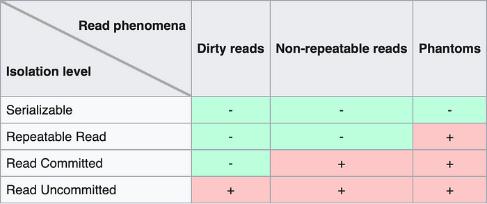
In our database, we will have a Serializable isolation level. Each transaction executes to completion before the next transaction begins.

We will achieve it by acquiring a RW lock before a transaction starts and releasing it when it ends. A RW lock can be held by an arbitrary number of readers or a single writer.

It means that our database can support a single writer or multiple readers at any given time, but not both.

Start Coding

DB

We will create a new file called db.go . We will add a new struct called DB and the methods Open and Close . DB contains dal and a RW lock. It manages access to the disk and ensures concurrent transactions don’t cause any anomalies, as described above.

DB is user-facing, so we will use public methods wrapping the dal layer.

We will also add two methods ReadTx and WriteTx for opening transactions and acquiring the lock.

Transactions

We will add a new file called tx.go . We will add a new tx struct and constructor.

The write flag indicates if the transaction is read-only or not. We will add a new error to const.go when a read-only transaction tries to make a change.

Then use it in the Put and Remove methods from earlier episodes.

Once a transaction starts, it either commits, and all modified data is saved, or it is rolled back, and all changes are ignored. Committing the changes is easy, as we have already done in previous parts, but rollback is more complicated.

Instead of reverting the changes when performing a rollback, an easier approach would be to store the modified nodes temporarily on RAM and propagate them to disk all at once. Then to perform a rollback, we have to do nothing since the data wasn’t committed.

For that, dirtyNodes holds modified nodes, waiting to be committed. pagesToDelete holds pages waiting to be deleted. And allocatedPageNums holds any new pageNums that we allocated by the freelist during the transaction.

If a transaction is read, performing a rollback is simple as only the mutex has to be released. If it’s a write transaction, we have to release pages given by the freelist , mark the slices as nil and release the mutex.

Performing a Commit is also straightforward. In a read transaction, only the mutex has to be released. In a write, modified nodes are saved, deleted nodes are removed, and any acquired pages are marked. Finally, the mutex is released.

Now we want to redirect the read/write/delete operations we added in previous episodes to dirtyNodes and pagesToDelete instead of the disk. It means that we will have to go over the code and replace accesses to dal to tx instead.

For example, do the following change:

Or the following inside the collection file:

This process is lengthy, but you can check all the changes on Github.

It’s important to notice that once we write a node, it’s not actually written to the disk but to a temporary buffer. If the system fails midway, we won’t be able to continue the transaction from the crash point.

To solve this problem, it’s possible to track the changes using WAL. It stands for write-ahead logging and is used for providing atomicity and durability. It’s usually implemented as an append-only log file recording changes to the database.

Then, every time the write node method is called (or delete), we could record the change in a separate log file (and not in the B-Tree!). If the system crashes, we could restore the database from the last call.

This is also out of the scope of our database, but our database is built so it can be easily extended with this improvement.

Chapter 6 Conclusion

In this part, we won’t showcase our new capabilities, but in the next part, we will have a working database from the bottom-up. We will add new methods for working with collections that will conclude all the critical features of our database.

Chapter 7

In this part, we will complete the database. We will take a deeper look at collections that we already saw before. This part is going to be our last episode as well.

Collections

We have already introduced the concept of collections. They store key-value pairs with a similar purpose and are the equivalent of an RDBMS table.

We discussed adding/removing/searching inside a given collection, but we haven’t discussed how to create them.

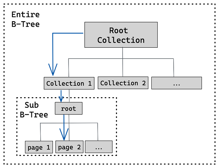
The idea is to have a master collection that holds other collections (Root Collection). It will contain key-value pairs, where the key is the collection name.

In a B-tree, every node is a root of a sub B-Tree so that every collection will be B-tree by itself and a sub B-tree of the entire B-Tree. The value will point to a page number that is the root of the collection sub-tree.

Remember that the meta page holds the page number of the B-tree root. The root field will point to the root page of the Root Collection.

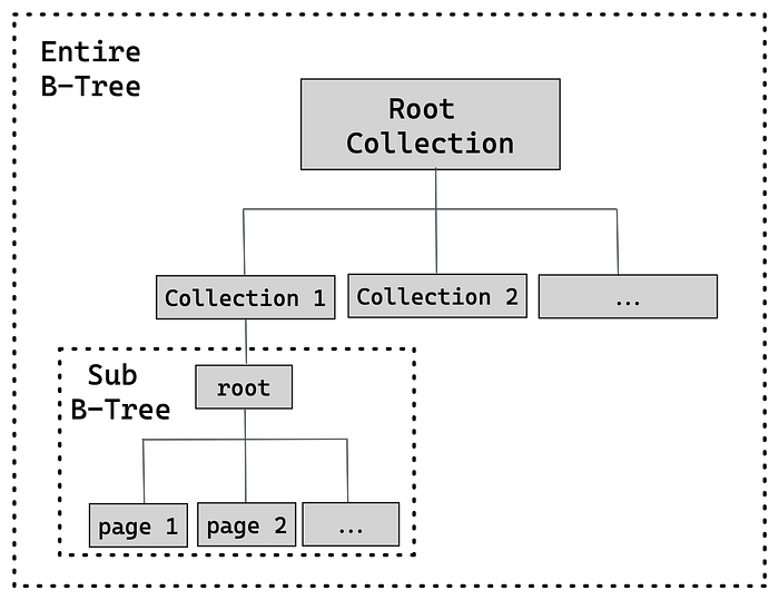
A real-life flow of searching a key-value pair in the database is as follows:

1. Start by retrieving the desired bucket to perform the search in. The database will search the Root Collection for the given collection.
2. Fetch the collection sub-tree root page
3. Find the desired element inside the collection sub-tree, starting at the root page.

Both steps 1 and 3 utilize the Find method we have implemented in part 4. The difference is the searched collection. The image below shows the process where each arrow corresponds to a step in the process.

Start Coding

We will start by implementing a method for retrieving the root collection. The critical part is assigning its root page the same as the entire DB’s root page.

Then we will add GetCollection as discussed above. Searching the root collection for the collection name, deserializing the content, and returning.

Creating and deleting a collection are similar. Apply Put /Remove on the Root Collection. Also, make sure the calling transaction is a write transaction.

Magic Numbers

We will add a final nice-to-have feature. A magic number is a constant numerical or text value used to identify a file format. Programs store in the first bytes an identifier such as CA FE BA BE (Java class files, for example). When the program loads, it compares the first bytes with the expected signature and ensures they are equal.

We will define our magic number to be D00DB00D (But it can be whatever you choose). We will include the magic number when writing the meta page to the disk. When loading it from the disk when the database starts, we will compare the file contents with the expected signature.

Chapter 7 Conclusion

This was a long journey, but our database is completed now. You should pat on your back if you followed me to this point.

To test our database, you can either use one of the tests inside the completed on Github or write your scenario. Any mix of read/write operations concurrently or non-concurrently will work.

Summary and Final Words

In chapter 1, we introduced broad terms such as SQL vs. NoSQL, data structures, and disk-based storage. We talked about our database, specifically the dal layer and its components, such as freelist and database pages.

Chapter 2 was all about persistence to the disk. We introduced a special page located on the file’s first page called meta. It holds all the information our database needs to start correctly. We also added methods for writing to the disk, such as: serialize /deserialize and read/write of meta and freelist pages. Those methods reappear every time a new entity is added to the database.

Chapter 3, 4, and 5 were about B-Trees. In chapter 3, we introduced binary search trees and talked about the rationale of B-Trees in databases. We decided to use slotted pages. A technique for organizing data on the disk by storing the data at the end of each page and fixed-size pointers to the data at the beginning.

Then, we started coding the B-Tree and finished that part with a search operation.

In chapter 4, we coded insertion to the database using B-Tree. We first saw the importance of keeping the B-Tree balanced and added methods for determining if the tree was out of balance- if it had too many/few elements in a node. Then we coded the split method to handle rebalancing and the insertion method itself. We also saw the collection entity for the first time.

In chapter 5, we finished coding the B-Tree by implementing the deletion and the appropriate balancing methods- left/right rotation and merge.

Chapter 6 differed from the previous parts since we weren’t handling disk operations. We brought up the topic of transactions- a work unit consisting of a sequence of operations performed on the database.

We talked about ACID- a set of properties for processing transactions reliably. We also looked closely at the isolation properly and used locks to ensure concurrent transactions don’t interfere with each other.

Finally, in chapter 7, we added the collections mechanism, the last piece remaining for the databases to function, and magic numbers that seal it completely.

Below you can see the general architecture of our database.

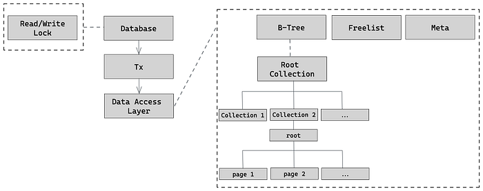
It was a year since I started writing the database till the articles were completed. I hope you enjoyed reading my posts half as much as I enjoyed writing them for you. Be sure to check the completed database called LibraDB on GitHub.