Boosting Machine Learning Performance With Rust
Rust + LibTorch = 5.5x training speed improvement on Python + PyTorch
In this article, I wish to share my experience of trying to create a little Machine Learning (ML) framework from scratch using Rust.
For my experiment, I had the following objectives in mind:
- I wanted to investigate whether rather than using Python + PyTorch, shifting to Rust + LibTorch (the C++ backend library of PyTorch) would translate into tangible speed improvements, especially during the model training process. As we know, ML models are becoming bigger and hence requiring increasing (sometimes unfeasible for the common bloke) computational power to train. One way to mitigate increasing hardware requirements is to identify a way how to make algorithms more computationally efficient. Knowing that within PyTorch, Python just acts as a layer on top of LibTorch, my big question was whether replacing the top Python layer with Rust is worth the effort. The plan was to use the
Tch-rsRust crate to just expose me to the Tensors and Autograd functionality of the LibTorch DLL, hence acting as our “gradients calculator”, but then develop the rest from scratch in Rust. - I wanted to keep the code simple enough to permit a clear understanding of all the linear algebra being performed and allow me to easily extend it if required.
- As much as possible my framework had to allow me to define ML models following a similar structure as per standard Python/PyTorch.
- Ummm … for “rusty” fun and learning :)
The post is not intended to teach Rust per se, but rather to provide an appreciation of how Rust can be applied for ML and the benefits of that.
Jumping straight to the final result, my little framework allows me to create Neural Network models as per below:
Listing 1 — Defining my Neural Network model.
struct MyModel {
    l1: Linear,
    l2: Linear,
}

impl MyModel {
    fn new (mem: &mut Memory) -> MyModel {
        let l1 = Linear::new(mem, 784, 128);
        let l2 = Linear::new(mem, 128, 10);
        Self {
            l1: l1,
            l2: l2,
        }
    }
}

impl Compute for MyModel {
    fn forward (&self,  mem: &Memory, input: &Tensor) -> Tensor {
        let mut o = self.l1.forward(mem, input);
        o = o.relu();
        o = self.l2.forward(mem, &o);
        o
    }
}
… and then instantiate and train the model like this:
Listing 2 — Instantiating and training my Neural Network model.
fn main() {
    let (x, y) = load_mnist();

    let mut m = Memory::new();
    let mymodel = MyModel::new(&mut m);
    train(&mut m, &x, &y, &mymodel, 100, 128, cross_entropy, 0.3);
    let out = mymodel.forward(&m, &x);
    println!("Training Accuracy: {}", accuracy(&y, &out));
}
For PyTorch users, the above creates quite an intuitive similarity with how one would define and train a Neural Network in Python. The example above shows a Neural Network model, which is then used for classification (the model is applied on the Mnist dataset, which I shall be using as my benchmark dataset to compare the Rust — Python model versions).
In the first block of the code, a MyModel struct is created which holds two layers of type Linear.
The second block is the MyModel stuct implementation, which defines an associated function new. This function initializes the two layers and returns a new instance of the struct.
Finally, the third block implements the Compute trait for MyModel, which defines the forward method. In the main function I then load the Mnist dataset, initialize the memory, instantiate MyModel, and then train it using 100 Epochs, batch size of 128, Cross Entropy Loss, and a learning rate of 0.3.
Pretty intuitive huh? That is what would be required to create and train new models in Rust using my little framework. However, we now start looking a bit under the hood to see what makes the above possible.
Looking at the above code, an obvious question might pop up if you are used to building ML models in PyTorch — what is the Memory reference doing? I explain below.
The Forward Pass
From ML literature, we know that the Neural Network training mechanism happens by iteratively going through two steps for a number of epochs (and normally also for a number of batches), a forward pass, and a backward pass (backpropagation).
In the forward pass, we push the inputs and subsequent calculations along all the layers in the network, where for each layer we have:
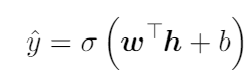
where w provides the weights for the linear function, b the biases, and then this is passed through an activation function such as Sigmoid providing the non-linearity.
With that information, we can now create our Linear layer (Listing 3 below). As you can notice, the structure for defining a layer follows the same structure for defining our model (Listing 1 above) and implements the same functions and traits.
In the case of the Linear layer, the struct contains a field named params. The params field is a collection of type HashMap, where the key is of type String, which stores a parameter name, and the value is of type usize, which holds the location of the specific parameter (which is a PyTorch tensor) in our Memory, which in turn acts as our store for all our parameters.
Listing 3— Defining a Neural Network Layer, in this case, a Linear Layer.
trait Compute {
    fn forward (&self,  mem: &Memory, input: &Tensor) -> Tensor;
}

struct Linear {
    params: HashMap<String, usize>,
}

impl Linear {
    fn new (mem: &mut Memory, ninputs: i64, noutputs: i64) -> Self {
        let mut p = HashMap::new();
        p.insert("W".to_string(), mem.new_push(&[ninputs,noutputs], true));
        p.insert("b".to_string(), mem.new_push(&[1, noutputs], true));

        Self {
            params: p,
        }
    }
}

impl Compute for Linear {
    fn forward (&self,  mem: &Memory, input: &Tensor) -> Tensor {
        let w = mem.get(self.params.get(&"W".to_string()).unwrap());
        let b = mem.get(self.params.get(&"b".to_string()).unwrap());
        input.matmul(w) + b
    }
}
In line with Equation 1, in our associated function new, we insert on our HashMap two parameters “W” and “b” that are required for the Linear Layer.
The mem.new_push() method, presented later, creates their respective tensors in the required sizes, pushes them to the memory store, and returns their location. The boolean parameter in the insert method defines that we need to calculate the gradient for these parameters. In this way, each layer will contain the parameter names and their respective tensor store locations in our Memory structure.
Similar to the MyModel definition, we then implement the Compute trait for our Linear Layer. This requires defining the function forward, which is called during the forward pass of the training process.
In this function, we first obtain a reference to the two tensor parameters from our tensor store using the get method and then calculate our linear function (Equation 1). Similar to PyTorch, from our Neural Network we output the unnormalized predictions (logits) and perform the normalization (in this case Softmax) later during the error calculation.
One might ask, why take this approach to represent a Linear Layer rather than maybe hard-coding Equation 1 directly in one or two lines of code?
This approach was taken so that if additional Neural Network layer types need to be defined, e.g. a CNN or an LSTM layer, then it is just a question of copying exactly the above Linear Layer structure and injecting additional parameters and computations in the associated function new and forward method and it will immediately become available to include in your models (as per Listing 1).
In addition, this approach of pushing all tensors in a central store will become handy in the backpropagation step, as I will discuss below.
Error Calculation
At the end of the forward pass, we need to calculate the error between our predictions and the targets.
Below is the code for mean squared error calculation, which is typically applied for regression, and cross-entropy loss, which is typically applied for classification.
Listing 4 — Mean Squared Error and Cross Entropy Loss Functions.
fn mse(target: &Tensor, pred: &Tensor) -> Tensor {
    (target - pred).square().mean(Kind::Float)
}

fn cross_entropy (target: &Tensor, pred: &Tensor) -> Tensor {
    let loss = pred.log_softmax(-1, Kind::Float).nll_loss(target);
    loss
}
And that completes the forward pass … we now kick off with the backward pass.
The Backward Pass
In the backward pass, we need to update the parameters of the model using the gradients, where each gradient is the derivative of the loss function with respect to each respective parameter. In the first step, we obtain the gradients:
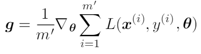
where m’ represents the size of the minibatch. For each minibatch, the parameters are then updated as follows:
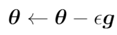
where epsilon is the learning rate.
This is where I use the Autograd functionality from LibTorch to obtain my gradients. In PyTorch, we normally apply the backward method on the loss to calculate the derivatives, which is then followed by calling the step function from the optimizer to apply the gradients to the model parameters. The same process happens here, with the difference that we cannot apply the step function directly to apply the gradients because we are not extending our models from the nn.Module class and using PyTorch optimizers as we normally do in Python. Hence the step part we need to cater to it ourselves.
In the snippet below (Listing 5) we show our tensor Memory implementation, which also caters to the gradient step functionality. The tensor store is implemented as a struct with two fields, a size, which holds the current number of tensors stored, and values, which is a vector of tensors. In the implementation block, the new method handles the store intialiazation and the push, new_push and get methods handle the passing back and forth of the tensors (the latter two we utilized in the Linear Layer above).
Listing 5 — The tensor store — Memory.
struct Memory {
    size: usize,
    values: Vec<Tensor>,
}

impl Memory {

    fn new() -> Self {
        let v = Vec::new();
        Self {size: 0,
            values: v}
    }

    fn push (&mut self, value: Tensor) -> usize {
        self.values.push(value);
        self.size += 1;
        self.size-1
    }

    fn new_push (&mut self, size: &[i64], requires_grad: bool) -> usize {
        let t = Tensor::randn(size, (Kind::Float, Device::Cpu)).requires_grad_(requires_grad);
        self.push(t)
    }

    fn get (&self, addr: &usize) -> &Tensor {
        &self.values[*addr]
    }

    fn apply_grads_sgd(&mut self, learning_rate: f32) {
        let mut g = Tensor::new();
        self.values
        .iter_mut()
        .for_each(|t| {
            if t.requires_grad() {
                g = t.grad();
                t.set_data(&(t.data() - learning_rate*&g));
                t.zero_grad();
            }
        });
    }

    fn apply_grads_sgd_momentum(&mut self, learning_rate: f32) {
        let mut g: Tensor = Tensor::new();
        let mut velocity: Vec<Tensor>= Tensor::zeros(&[self.size as i64], (Kind::Float, Device::Cpu)).split(1, 0);
        let mut vcounter = 0;
        const BETA:f32 = 0.9;

        self.values
        .iter_mut()
        .for_each(|t| {
            if t.requires_grad() {
                g = t.grad();
                velocity[vcounter] = BETA * &velocity[vcounter] + (1.0 - BETA) * &g;
                t.set_data(&(t.data() - learning_rate * &velocity[vcounter]));
                t.zero_grad();
            }
            vcounter += 1;
        });
    }
}
The last two methods in the code above implement the basic gradient descent and the gradient descent with momentum algorithms. The methods assume that the backward step, which generates the gradients, was already called, so here we are handling what in PyTorch would be the step function call.
The process involves looping through each tensor on the store, obtain the calculated gradient using the grad method, and then by calling the set_data method we apply the parameter update rule. One can easily introduce other methods and implement other algorithms such as Rmsprop and Adam.
The Training Loop
In the training loop, we bring together everything discussed earlier for our learning process. As usual, we apply a loop for each epoch, in which we are then looping for each minibatch, and for each minibatch we do a forward pass, calculate the error, call the backward method on the error to generate the gradients, and then apply the gradients (Listing 6).
Listing 6— The training loop.
fn train<F>(mem: &mut Memory, x: &Tensor, y: &Tensor, model: &dyn Compute, epochs: i64, batch_size: i64, errfunc: F, learning_rate: f32)
    where F: Fn(&Tensor, &Tensor)-> Tensor
        {
        let mut error = Tensor::from(0.0);
        let mut batch_error = Tensor::from(0.0);
        let mut pred = Tensor::from(0.0);
        for epoch in 0..epochs {
            batch_error = Tensor::from(0.0);
            for (batchx, batchy) in get_batches(&x, &y, batch_size, true) {
                pred = model.forward(mem, &batchx);
                error = errfunc(&batchy, &pred);
                batch_error += error.detach();
                error.backward();
                mem.apply_grads_sgd_momentum(learning_rate);
            }
            println!("Epoch: {:?} Error: {:?}", epoch, batch_error/batch_size);
        }
}
Whilst in PyTorch we have our Dataset and Dataloader classes which handle the data mini-batching mechanism, in my case I built my own batching mechanism.
The Rust function below (Listing 7) accepts a reference to the full dataset and then returns an iterator which allows the training function (Listing 6) to iterate over the mini-batches.
Listing 7— Mini-batching.
fn get_batches(x: &Tensor, y: &Tensor, batch_size: i64, shuffle: bool) -> impl Iterator<Item = (Tensor, Tensor)> {
    let num_rows = x.size()[0];
    let num_batches = (num_rows + batch_size - 1) / batch_size;

    let indices = if shuffle {
        Tensor::randperm(num_rows as i64, (Kind::Int64, Device::Cpu))
    } else
    {
        let rng = (0..num_rows).collect::<Vec<i64>>();
        Tensor::from_slice(&rng)
    };
    let x = x.index_select(0, &indices);
    let y = y.index_select(0, &indices);

    (0..num_batches).map(move |i| {
        let start = i * batch_size;
        let end = (start + batch_size).min(num_rows);
        let batchx: Tensor = x.narrow(0, start, end - start);
        let batchy: Tensor = y.narrow(0, start, end - start);
        (batchx, batchy)
    })
}
Final Helper Functions
The last two functions that you will need to run the full code, are just two helper functions (Listing 8).
The first function loads the dataset from a directory that I named data (you have to first download the Mnist dataset).
The second function calculates the accuracy of the model, accepting as parameters a reference to the target and predictions.
Listing 8 — Last two helper functions.
fn load_mnist() -> (Tensor, Tensor) {
    let m = vision::mnist::load_dir("data").unwrap();
    let x = m.train_images;
    let y = m.train_labels;
    (x, y)
}

fn accuracy(target: &Tensor, pred: &Tensor) -> f64 {
    let yhat = pred.argmax(1,true).squeeze();
    let eq = target.eq_tensor(&yhat);
    let accuracy: f64 = (eq.sum(Kind::Int64) / target.size()[0]).double_value(&[]).into();
    accuracy
}
The only imports that you will need are:
Listing 9 — Required imports.
use std::{collections::HashMap};
use tch::{Tensor, Kind, Device, vision, Scalar};
Before running the code you also need to download the LibTorch C++ Library from the PyTorch website.
Results and Opinions
To compare the above code with a Python-PyTorch equivalent, I tried to be as faithful as possible to get a fair comparison, mainly ensuring that I apply the same Neural Network hyper-parameters, training parameters, and training algorithms.
For my tests, I applied the Mnist dataset, which consists of 60K training examples with 28x28 features. I ran the tests on my laptop, a Surface Pro 8, i7, with 16G of RAM, hence no GPU. After running the tests multiple times, on average Rust training resulted in 5.5 times faster than the Python equivalent. Unfortunately, at this point I didn’t pinpoint which areas in the training process generated the biggest gains in performance over and above a standard PyTorch approach (is it in the training loops?, in the error calculations?, in the gradient step?, etc), hence the gain I mention is an overall gain over the whole process.
As a concluding thought, developing the above in Rust definitely takes more time initially, especially for someone like me who I still consider a newbie in Rust, however, once you build all your library components and pipeline code and just need to test/create new models (like in Listing 1), then in my opinion it becomes as easy as working in Python.
The improvements in training speed that I experienced are in my opinion not to be ignored — it could literally save long hours, if not days, of training, especially with the increasing complexity of ML models, larger datasets, or huge iterative learning processes like in Reinforcement Learning.
Hope you found the article worth the read! In our Part 2 of the series we focus on Convolutional Neural Networks.
References
Ian Goodfellow, Yoshua Bengio and Aaron Courville, Deep Learning, MIT Press, 2016. http://www.deeplearningbook.org