A Quick Look at D3.js
Visualize anything you dream of using the power of JavaScript
D3, short for Data-Driven Documents, is a JavaScript library that makes it possible to display data in a multitude of ways and helps with inspection and manipulation of the DOM.
Although you may think it is, D3 is not a charting library. It offers much more flexibility, which is leveraged by existing charting libraries like Recharts, C3js, and Raw graphs. D3 is great because where your charting library breaks down when you’re trying to customize it too much, D3 just keeps ongoing.
In this article, you’ll get to know D3 using examples. The general flow can be boiled down to:

But first, let’s start by drawing some different colored shapes to a webpage. This will get you accustomed to using selectors and shapes.
Draw Basic Shapes
So how exactly can we draw using D3? We’ll start by creating an HTML page that contains an empty SVG (scalable vector graphic). If you don’t know what an SVG is, it’s an image that is made up out of primary shapes, which makes it very scalable. We will be drawing these primary shapes using D3.
First, create an HTML document that imports D3. We will keep using this same HTML document throughout this whole article. We’ll only edit the code between the script tags that are highlighted.

So as you can see, on line 4 we’ve imported D3. If you’re using a frontend framework with Node.js, you can use NPM. On line 7 we’ve defined an SVG element in which we will draw our shapes.
Let’s write our first lines of D3 code:

On line 2, we start by using the d3.select() method. This selector function will look for the first element with the CSS selector that you passed to the function. In our case, there is only one <svg> tag on the page, so it will return the only existing SVG element.
Another selector function that we’ll use later is d3.selectAll(). This function will return all elements matching the CSS selector instead of just the first one.
On line 4 we use the SVG element and append a circle to it. You can add a multitude of different shapes to the SVG element. On line 5, we apply D3’s method chaining. Method chaining allows us to call multiple functions one after the other, preventing us from having to write svg.function(...) on every single line.
On lines 5, 6, 7, and 8 we set attributes using the d3.attr function. These attributes are necessary to visualize our circle. cx will be the x coordinate of the center of our circle, cy will be the y coordinate of the center, r will be the radius of the circle, and fill will be the color the circle will be filled with. These are fixed attributes. Examples of the usages of these attributes for every basic shape can be found on freeCopeCamp.
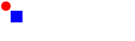
So finally, if you look into your browser, you’ll see something like this:

This may not seem like much, but it’s great. Even the most complicated graphs are just a bunch of simple shapes.
Let’s add another square to the image:
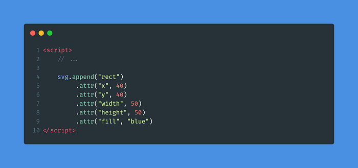
We append a rect shape and set the attributes necessary for displaying it correctly. Running the code gives us the following result:
Now that you know the basics of adding shapes, let’s get started by loading in some data and displaying shapes depending on that data.
Load Data
There are multiple D3 functions for fetching different types of data. The most interesting ones to start are d3.json('...'), d3.csv('...'), and d3.xml('...').
All three use Fetch under the hood to “fetch” the data. CSV doesn’t allow for nested objects, while JSON and XML do.
For the coming chapters, we will use the following data file from our imaginary social network (socialnetwork.json) and the following styles:


We’re going to start by building a graph chart for the library. Horizontally we’ll display our years, and vertically we’ll display our number of comments. We’ll do this by using d3.axisBottom() and d3.axisLeft(), respectively. In code, loading our data and drawing our axis goes like this:

That’s a lot of code! No worries, we’ll go through it line by line.
On line 3 we start by fetching our JSON, as d3.json() returns a promise we have to use .then() or await to wait for the fetch to complete. Once it’s done on lines 5 and 10, we start by creating scale functions.
Scale functions
Scale functions are one of the keys to rendering our data to our screen. Assume that we have years spreading from 2015–2020 and a screen resolution of 500 x 500. If we display the year number on the x-axis, we want to map 2015–2020 to 0–500.
That’s where scale functions come in. One of them is .scaleLinear(), which will linearly convert a range of numbers to a different range. To the scaleLinear() function we give a range on Line 7. We pass a range [100,800] because I want to start drawing on the 100th pixel and end drawing on the 800th pixel on the x-axis.
After that, we pass a domain, which is the range of the data we want to map. .domain() expects an array with a minimum and a maximum. Luckily for us, D3 has the functions d3.extent(), d3.max(), and d3.min(). On line 8, we set the minimum to the minimum of years — 1 and the maximum to maximum of years + 1. We do this to be able to center our bars in the bar chart later on.
On line 13, I do something slightly different because I want the axis to start at 0 and end at the maximum of comments instead. I don’t want to show the comments range 50–150, but I want to show the comments from 0–150.
d3.extent() will figure return [max, min] without you having to call min and max separately.
Then it’s time to draw the actual axis. On line 15 we start by adding the x-axis. We give it a class for styling purposes (see the styling image) and then we translate our g-element because an x-axis always draws from the origin, which is top left. So we translate it to the bottom instead. After that we execute .call(d3.axisBottom(x).tickFormat(d3.format("d")). .axisBottom will draw our axis. (Note that we give it the range function, so it knows in what range/domain to execute.) Then we do an additional .tickFormat(), which tells D3 how to display the labels. In our case we want simple numbers ranging from 2014–2021, so we use "d".
After that, we do basically the same thing for the y-axis, except that the transform is different because we need to translate the axis horizontally to display the labels.
The result is something like this:

Select Elements and Bind Data
Next, we want to draw rectangles for every year based on the number of comments. For this, we will select our SVG and bind our data.
This boils down to writing something like this:
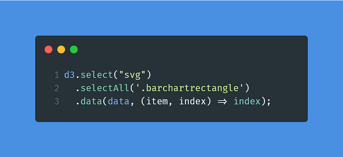
First, we use the d3.select() function to get our SVG. (Note that in the prior code snippets, we saved this in a variable called svg.) We then select all existing bar chart rectangles by searching with the CSS “selector .barchartrectangle.” This is for updating purposes: If the array changes, we want to select the existing rectangles to update/remove them.
After that, we call the .data() function. The data function itself has one mandatory argument, which is the data you’ll want to render, and a second optional argument that specifies the key. To specify the key, we give it a function that accepts an item and the index in the array. In this example, I return the index.
However! As we will see in the coming part, you might use a field on the item to know which items to update/remove/insert. If we have an id property in our dataset, we could write something like (item, index)=> item.id.
So now that we know how to data-bind, let’s append some rectangles.
Create, Update, and Remove Elements
When you update the data in your array (e.g., by filtering) D3 will compare arrays and decide what to do.
For now, I will only go over the two most important functions: addition .enter() and removal .exit().
To understand the logic, consider the following code:
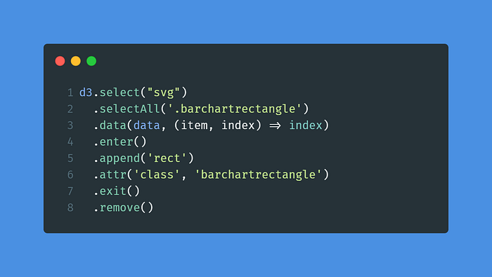
Consider that we’re using this array as data [1,2,3] when we first execute this code.
Our selector .barchartrectangle will return 0 elements, so D3 knows that the items in our array are three new pieces of data. Therefore it will use the functions changed to the .enter() statement. In this statement we append new rects for every new piece of data and give them the class barchartrectangle. Since there are no “deletions,” the .exit() statement will be neglected.
Now if we update our array to [1,2] and run this code again, the .barchartrectangle selector will return three existing elements. However, D3 noticed that there are only two items in the array. So it will use the functions chained to the .exit() statement, and in this case, .remove() the third element.
How does D3 know what elements to delete? That depends on the data key we defined earlier. In our case, this is still the index, so it will remove the third element it had added. However, if our item was the actual id (item, index)=> item and we updated the array to [1,3], then our second barchartrectangle would be removed instead of our third one.
Now that you know how the .enter() and .exit() statements work, it’s time to render our bar chart.
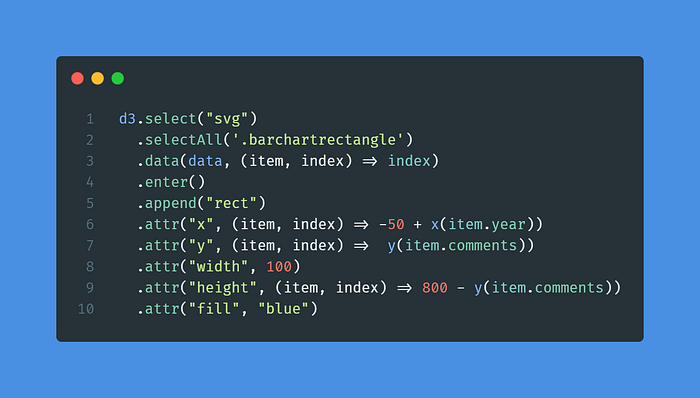
On line 4, we start by using .enter() so that D3 will know what to do with new data. On line 5, we append a new rect, after which we set all the necessary attributes. As you can see on lines 6 and 7, the .attr() function doesn’t only take fixed values; instead, it can take a function that uses the item and its index. This way we can draw our elements depending on our data.
On line 6, we first get the scaled x position by calling our x scaling function defined earlier with our year. This will return the pixel value we want to place our bar chart on. As we will set the width to 100 later, we adjust the bar to the center of the value point by doing -50 . For the y coordinate, we can simply call our scaling function. For the height on line 9, we have to do 800- y(item.comments). That’s because our scaling function was inverse. Remember our range was [800, 100, so low comment values will be mapped to a high pixel value. That’s why we have to inverse it by doing 800 — y(item.comments).
Lastly, we set the fill color to blue, just for esthetics. The final result is:
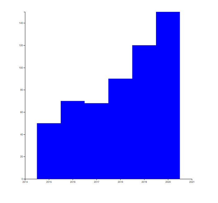
There you are — we rendered something to our screen using data. That’s what D3 is all about! But remember there’s much more to do. Check out the cool charts and figures on D3.js — Data-Driven Documents (d3js.org).
If you want to understand D3 in more depth or get more great examples, I recommend the book D3.js in Action by Elijah Meeks.
Conclusion
In this article, you got a quick introduction to rendering using the D3 library. You can now visualize shapes in an SVG using dynamically generated data.
There’s still plenty to learn: geo-mapping, HTML manipulation, network visualization…. The list goes on. But one great thing about 3D is that there are almost no boundaries. So go ahead and try it out!

